Utah Census Data: Measles Outbreak Modeling Comparison
utah_census_comparison.Rmd
library(multigroup.vaccine)
library(socialmixr)

# Use the included example data file to avoid download issues during package building
census_csv <- getCensusDataPath()
Introduction
This vignette demonstrates how to use the
getCensusData() function to retrieve real U.S. Census
Bureau population data for Utah counties and use it in measles outbreak
modeling. We’ll compare how different counties with varying demographic
structures respond to measles outbreaks under different vaccination
scenarios.
Note: This vignette uses the included example census data file to ensure it works offline and during package building.
Measles Model Setup
For measles outbreak modeling, we’ll use the standard age groups from the measles age-structured model:
Getting Census Data for Utah Counties
Let’s retrieve population data for three diverse Utah counties:
utah_fips <- getStateFIPS("Utah")

# Get data for three counties with different characteristics
counties <- c("Salt Lake County", "Utah County", "Washington County")

county_data_list <- list()

for (county in counties) {
  data <- getCensusData(
    state_fips = utah_fips,
    county_name = county,
    year = 2024,
    age_groups = agelims,
    csv_path = census_csv
  )

  county_data_list[[county]] <- data

  cat("\n", county, ":\n", sep = "")
  cat("  Total population:", format(data$total_pop, big.mark = ","), "\n")
  cat("  Age distribution:\n")
  for (i in seq_along(data$age_labels)) {
    pct <- 100 * data$age_pops[i] / data$total_pop
    cat(sprintf("    %s: %s (%.1f%%)\n",
                data$age_labels[i],
                format(data$age_pops[i], big.mark = ","),
                pct))
  }
}
#> Reading census data from: /home/runner/work/_temp/Library/multigroup.vaccine/extdata/cc-est2024-syasex-49.csv
#> Aggregating ages 0 to 0: sum = 14732
#> Aggregating ages 1 to 4: sum = 57711
#> Aggregating ages 5 to 11: sum = 111884
#> Aggregating ages 12 to 17: sum = 108100
#> Aggregating ages 18 to 24: sum = 125472
#> Aggregating ages 25 to 44: sum = 379015
#> Aggregating ages 45 to 69: sum = 318909
#>
#> Salt Lake County:
#>   Total population: 1,216,274
#>   Age distribution:
#>     under1: 14,732 (1.2%)
#>     1to4: 57,711 (4.7%)
#>     5to11: 111,884 (9.2%)
#>     12to17: 108,100 (8.9%)
#>     18to24: 125,472 (10.3%)
#>     25to44: 379,015 (31.2%)
#>     45to69: 318,909 (26.2%)
#>     70plus: 100,451 (8.3%)
#> Reading census data from: /home/runner/work/_temp/Library/multigroup.vaccine/extdata/cc-est2024-syasex-49.csv
#> Aggregating ages 0 to 0: sum = 12053
#> Aggregating ages 1 to 4: sum = 48596
#> Aggregating ages 5 to 11: sum = 88402
#> Aggregating ages 12 to 17: sum = 78366
#> Aggregating ages 18 to 24: sum = 125580
#> Aggregating ages 25 to 44: sum = 210551
#> Aggregating ages 45 to 69: sum = 143596
#>
#> Utah County:
#>   Total population: 747,234
#>   Age distribution:
#>     under1: 12,053 (1.6%)
#>     1to4: 48,596 (6.5%)
#>     5to11: 88,402 (11.8%)
#>     12to17: 78,366 (10.5%)
#>     18to24: 125,580 (16.8%)
#>     25to44: 210,551 (28.2%)
#>     45to69: 143,596 (19.2%)
#>     70plus: 40,090 (5.4%)
#> Reading census data from: /home/runner/work/_temp/Library/multigroup.vaccine/extdata/cc-est2024-syasex-49.csv
#> Aggregating ages 0 to 0: sum = 2263
#> Aggregating ages 1 to 4: sum = 9687
#> Aggregating ages 5 to 11: sum = 18808
#> Aggregating ages 12 to 17: sum = 18446
#> Aggregating ages 18 to 24: sum = 19948
#> Aggregating ages 25 to 44: sum = 49399
#> Aggregating ages 45 to 69: sum = 55271
#>
#> Washington County:
#>   Total population: 207,943
#>   Age distribution:
#>     under1: 2,263 (1.1%)
#>     1to4: 9,687 (4.7%)
#>     5to11: 18,808 (9.0%)
#>     12to17: 18,446 (8.9%)
#>     18to24: 19,948 (9.6%)
#>     25to44: 49,399 (23.8%)
#>     45to69: 55,271 (26.6%)
#>     70plus: 34,121 (16.4%)
Scenario 1: Current Vaccination Coverage
Let’s model outbreaks under current estimated vaccination coverage levels in Utah.
# Based on school data and estimates
current_coverage <- c(0, 0.89, 0.949, 0.950, 0.95, 0.95, 0.95, 1)
Salt Lake County - Current Coverage
slc_data <- county_data_list[["Salt Lake County"]]

slc_current <- multigroup.vaccine:::getOutputTable(
  agelims = agelims,
  agepops = slc_data$age_pops,
  agecovr = current_coverage,
  ageveff = ageveff,
  initgrp = initgrp
)

cat("Salt Lake County - Current Vaccination Coverage\n")
#> Salt Lake County - Current Vaccination Coverage
print(as.data.frame(slc_current), row.names = FALSE)
#>  R0  R0local        Rv pEscape escapeInfTot under1 1to4 5to11 12to17 18to24
#>  10 11.42435 0.9402893   0.000            0      0    0     0      0      0
#>  11 12.56679 1.0343182   0.075         4922    400  448   599    846    508
#>  12 13.70922 1.1283471   0.093        17506   1530 1654  2070   2638   1812
#>  13 14.85166 1.2223761   0.146        28583   2644 2760  3275   3908   2954
#>  14 15.99409 1.3164050   0.239        38133   3694 3727  4241   4838   3926
#>  15 17.13653 1.4104339   0.272        46321   4661 4559  5015   5539   4748
#>  16 18.27896 1.5044628   0.287        53345   5544 5269  5639   6078   5440
#>  17 19.42140 1.5984918   0.347        59386   6345 5875  6146   6501   6026
#>  18 20.56383 1.6925207   0.380        64604   7069 6392  6560   6837   6522
#>  25to44 45to69 70+
#>       0      0   0
#>    1375    746   0
#>    5014   2788   0
#>    8306   4736   0
#>   11175   6530   0
#>   13640   8158   0
#>   15747   9627   0
#>   17546  10948   0
#>   19086  12137   0
Utah County - Current Coverage
utah_data <- county_data_list[["Utah County"]]

utah_current <- multigroup.vaccine:::getOutputTable(
  agelims = agelims,
  agepops = utah_data$age_pops,
  agecovr = current_coverage,
  ageveff = ageveff,
  initgrp = initgrp
)

cat("\nUtah County - Current Vaccination Coverage\n")
#>
#> Utah County - Current Vaccination Coverage
print(as.data.frame(utah_current), row.names = FALSE)
#>  R0  R0local       Rv pEscape escapeInfTot under1 1to4 5to11 12to17 18to24
#>  10 13.36528 1.106482   0.101         9582    983 1126  1361   1603   1614
#>  11 14.70180 1.217131   0.129        18227   2025 2219  2503   2724   3042
#>  12 16.03833 1.327779   0.206        25527   3016 3168  3391   3507   4210
#>  13 17.37486 1.438427   0.251        31653   3929 3970  4080   4075   5157
#>  14 18.71139 1.549075   0.276        36800   4754 4640  4618   4499   5924
#>  15 20.04792 1.659724   0.348        41143   5495 5198  5043   4821   6549
#>  16 21.38444 1.770372   0.355        44826   6156 5663  5381   5071   7060
#>  17 22.72097 1.881020   0.394        47967   6745 6051  5654   5267   7482
#>  18 24.05750 1.991668   0.406        50660   7269 6378  5875   5423   7831
#>  25to44 45to69 70+
#>    2025    870   0
#>    3967   1747   0
#>    5671   2563   0
#>    7136   3306   0
#>    8386   3978   0
#>    9452   4585   0
#>   10362   5133   0
#>   11140   5628   0
#>   11808   6075   0
Washington County - Current Coverage
wash_data <- county_data_list[["Washington County"]]

wash_current <- multigroup.vaccine:::getOutputTable(
  agelims = agelims,
  agepops = wash_data$age_pops,
  agecovr = current_coverage,
  ageveff = ageveff,
  initgrp = initgrp
)

cat("\nWashington County - Current Vaccination Coverage\n")
#>
#> Washington County - Current Vaccination Coverage
print(as.data.frame(wash_current), row.names = FALSE)
#>  R0  R0local        Rv pEscape escapeInfTot under1 1to4 5to11 12to17 18to24
#>  10 10.86329 0.8823416   0.000            0      0    0     0      0      0
#>  11 11.94962 0.9705758   0.000            0      0    0     0      0      0
#>  12 13.03595 1.0588100   0.079         1130     86  109   153    231    117
#>  13 14.12227 1.1470441   0.112         2737    225  276   363    493    285
#>  14 15.20860 1.2352783   0.140         4217    369  437   545    687    441
#>  15 16.29493 1.3235125   0.204         5541    509  585   696    834    580
#>  16 17.38126 1.4117466   0.255         6711    642  716   820    946    701
#>  17 18.46759 1.4999808   0.268         7741    767  831   922   1035    806
#>  18 19.55392 1.5882150   0.322         8647    882  931  1006   1104    898
#>  25to44 45to69 70+
#>       0      0   0
#>       0      0   0
#>     250    184   0
#>     625    469   0
#>     984    754   0
#>    1312   1026   0
#>    1605   1281   0
#>    1865   1516   0
#>    2092   1733   0
Visualization: Comparing Counties
Let’s visualize the outbreak potential across counties:
# Extract R0=15 results for comparison
r0_15_idx <- which(slc_current[, "R0"] == 15)

counties_names <- c("Salt Lake", "Utah", "Washington")
escape_totals <- c(
  slc_current[r0_15_idx, "escapeInfTot"],
  utah_current[r0_15_idx, "escapeInfTot"],
  wash_current[r0_15_idx, "escapeInfTot"]
)
total_pops <- c(
  slc_data$total_pop,
  utah_data$total_pop,
  wash_data$total_pop
)

escape_pcts <- 100 * escape_totals / total_pops

par(mfrow = c(1, 2), mar = c(5, 4, 4, 2))

# Absolute numbers
barplot(escape_totals,
        names.arg = counties_names,
        main = "Potential Outbreak Size (R0=15)\nCurrent Coverage",
        ylab = "Total Infections",
        col = "coral",
        las = 2)

# Percentages
barplot(escape_pcts,
        names.arg = counties_names,
        main = "% of Population (R0=15)\nCurrent Coverage",
        ylab = "% of Population Infected",
        col = "steelblue",
        las = 2)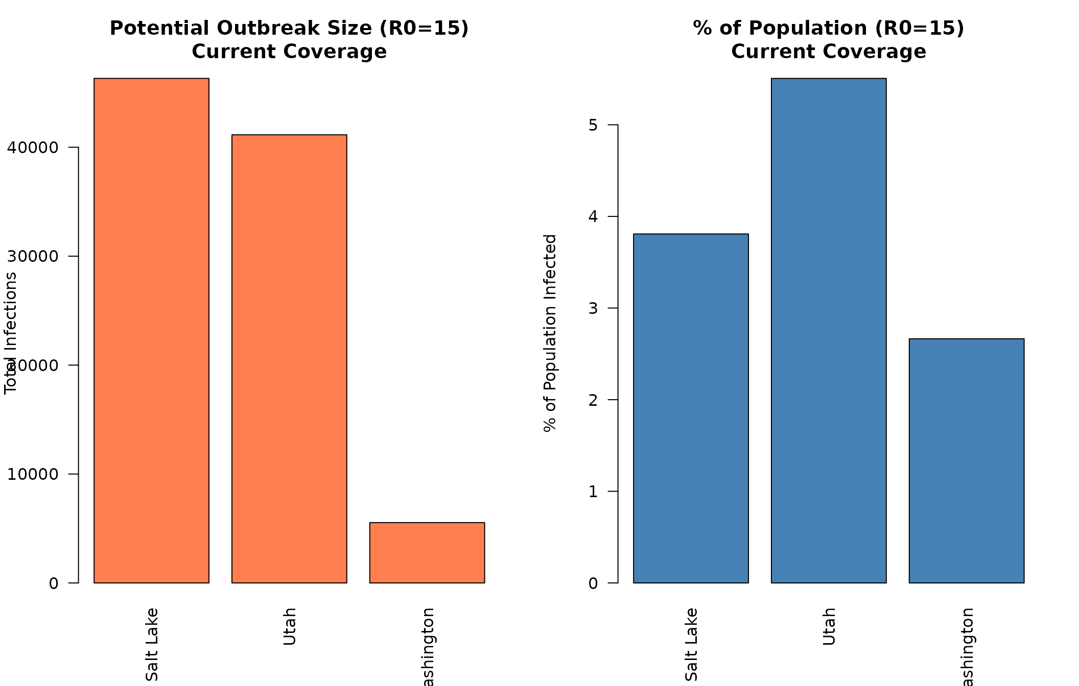
Scenario 2: Reduced Vaccination Coverage
What happens if vaccination coverage drops by 10% across all age groups?
reduced_coverage <- current_coverage * 0.9  # 10% reduction
reduced_coverage[1] <- 0  # Keep under-1 at 0
slc_reduced <- multigroup.vaccine:::getOutputTable(
  agelims = agelims,
  agepops = slc_data$age_pops,
  agecovr = reduced_coverage,
  ageveff = ageveff,
  initgrp = initgrp
)

utah_reduced <- multigroup.vaccine:::getOutputTable(
  agelims = agelims,
  agepops = utah_data$age_pops,
  agecovr = reduced_coverage,
  ageveff = ageveff,
  initgrp = initgrp
)

wash_reduced <- multigroup.vaccine:::getOutputTable(
  agelims = agelims,
  agepops = wash_data$age_pops,
  agecovr = reduced_coverage,
  ageveff = ageveff,
  initgrp = initgrp
)

cat("Salt Lake County - Reduced Coverage (-10%)\n")
#> Salt Lake County - Reduced Coverage (-10%)
print(as.data.frame(slc_reduced), row.names = FALSE)
#>  R0  R0local       Rv pEscape escapeInfTot under1  1to4 5to11 12to17 18to24
#>  10 11.42435 1.979104   0.455       149540   7095 10043 15806  16378  16556
#>  11 12.56679 2.177015   0.487       161833   8031 10966 16683  16985  17699
#>  12 13.70922 2.374925   0.535       171440   8836 11687 17311  17399  18545
#>  13 14.85166 2.572836   0.569       179053   9532 12255 17768  17688  19180
#>  14 15.99409 2.770746   0.608       185157  10135 12706 18105  17892  19662
#>  15 17.13653 2.968657   0.634       190105  10660 13067 18357  18038  20032
#>  16 18.27896 3.166567   0.663       194153  11118 13358 18547  18144  20319
#>  17 19.42140 3.364477   0.682       197493  11519 13594 18691  18222  20542
#>  18 20.56383 3.562388   0.689       200269  11871 13787 18801  18279  20717
#>  25to44 45to69  70+
#>   47891  32417 3355
#>   51657  35938 3873
#>   54497  38823 4342
#>   56661  41202 4767
#>   58327  43176 5154
#>   59620  44824 5507
#>   60632  46206 5829
#>   61428  47372 6125
#>   62059  48358 6397
Impact of Reduced Coverage
# Compare current vs reduced for R0=15
escape_reduced <- c(
  slc_reduced[r0_15_idx, "escapeInfTot"],
  utah_reduced[r0_15_idx, "escapeInfTot"],
  wash_reduced[r0_15_idx, "escapeInfTot"]
)

comparison_matrix <- rbind(escape_totals, escape_reduced)
colnames(comparison_matrix) <- counties_names
rownames(comparison_matrix) <- c("Current", "Reduced -10%")

barplot(comparison_matrix,
        beside = TRUE,
        main = "Impact of 10% Reduction in Vaccination Coverage\n(R0=15)",
        xlab = "County",
        ylab = "Total Infections",
        col = c("steelblue", "coral"),
        legend.text = rownames(comparison_matrix),
        args.legend = list(x = "topleft", bty = "n"))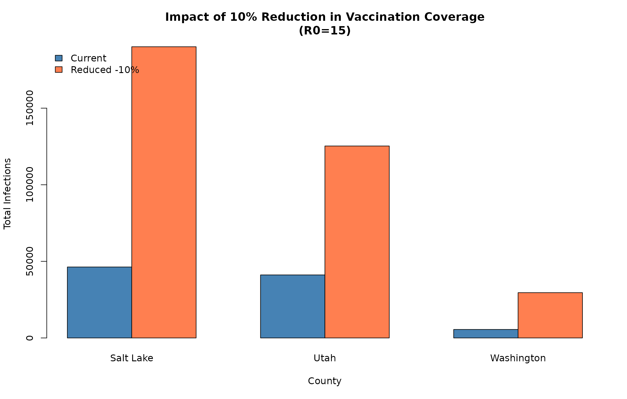
# Calculate percent increase
pct_increase <- 100 * (escape_reduced - escape_totals) / escape_totals
cat("\nPercent increase in outbreak size with 10% coverage reduction:\n")
#>
#> Percent increase in outbreak size with 10% coverage reduction:
for (i in seq_along(counties_names)) {
  cat(sprintf("  %s: +%.1f%%\n", counties_names[i], pct_increase[i]))
}
#>   Salt Lake: +310.4%
#>   Utah: +204.6%
#>   Washington: +433.7%
Scenario 3: Age-Specific Vaccination Gaps
What if vaccination coverage is particularly low in school-age children (5-17)?
school_gap_coverage <- current_coverage
school_gap_coverage[3] <- 0.75  # 5-11: reduced from 85.2% to 75%
school_gap_coverage[4] <- 0.75  # 12-17: reduced from 87.9% to 75%
slc_schoolgap <- multigroup.vaccine:::getOutputTable(
agelims = agelims,
agepops = slc_data$age_pops,
agecovr = school_gap_coverage,
ageveff = ageveff,
initgrp = initgrp
)
utah_schoolgap <- multigroup.vaccine:::getOutputTable(
agelims = agelims,
agepops = utah_data$age_pops,
agecovr = school_gap_coverage,
ageveff = ageveff,
initgrp = initgrp
)
wash_schoolgap <- multigroup.vaccine:::getOutputTable(
agelims = agelims,
agepops = wash_data$age_pops,
agecovr = school_gap_coverage,
ageveff = ageveff,
initgrp = initgrp
)
cat("Salt Lake County - School-Age Vaccination Reduction\n")
#> Salt Lake County - School-Age Vaccination Reduction
print(as.data.frame(slc_schoolgap), row.names = FALSE)
#> R0 R0local Rv pEscape escapeInfTot under1 1to4 5to11 12to17 18to24
#> 10 11.42435 2.612491 0.344 95041 4956 5198 26503 27594 5429
#> 11 12.56679 2.873740 0.371 101832 5740 5820 27564 28171 6022
#> 12 13.70922 3.134989 0.411 107627 6480 6367 28326 28561 6540
#> 13 14.85166 3.396238 0.452 112603 7173 6843 28880 28829 6990
#> 14 15.99409 3.657487 0.487 116895 7816 7257 29286 29015 7379
#> 15 17.13653 3.918736 0.482 120612 8409 7614 29585 29144 7715
#> 16 18.27896 4.179985 0.569 123841 8954 7923 29807 29235 8003
#> 17 19.42140 4.441234 0.568 126656 9453 8190 29973 29299 8252
#> 18 20.56383 4.702483 0.600 129117 9909 8420 30097 29344 8465
#> 25to44 45to69 70+
#> 15880 9481 0
#> 17706 10810 0
#> 19308 12044 0
#> 20705 13182 0
#> 21917 14226 0
#> 22966 15179 0
#> 23871 16048 0
#> 24653 16838 0
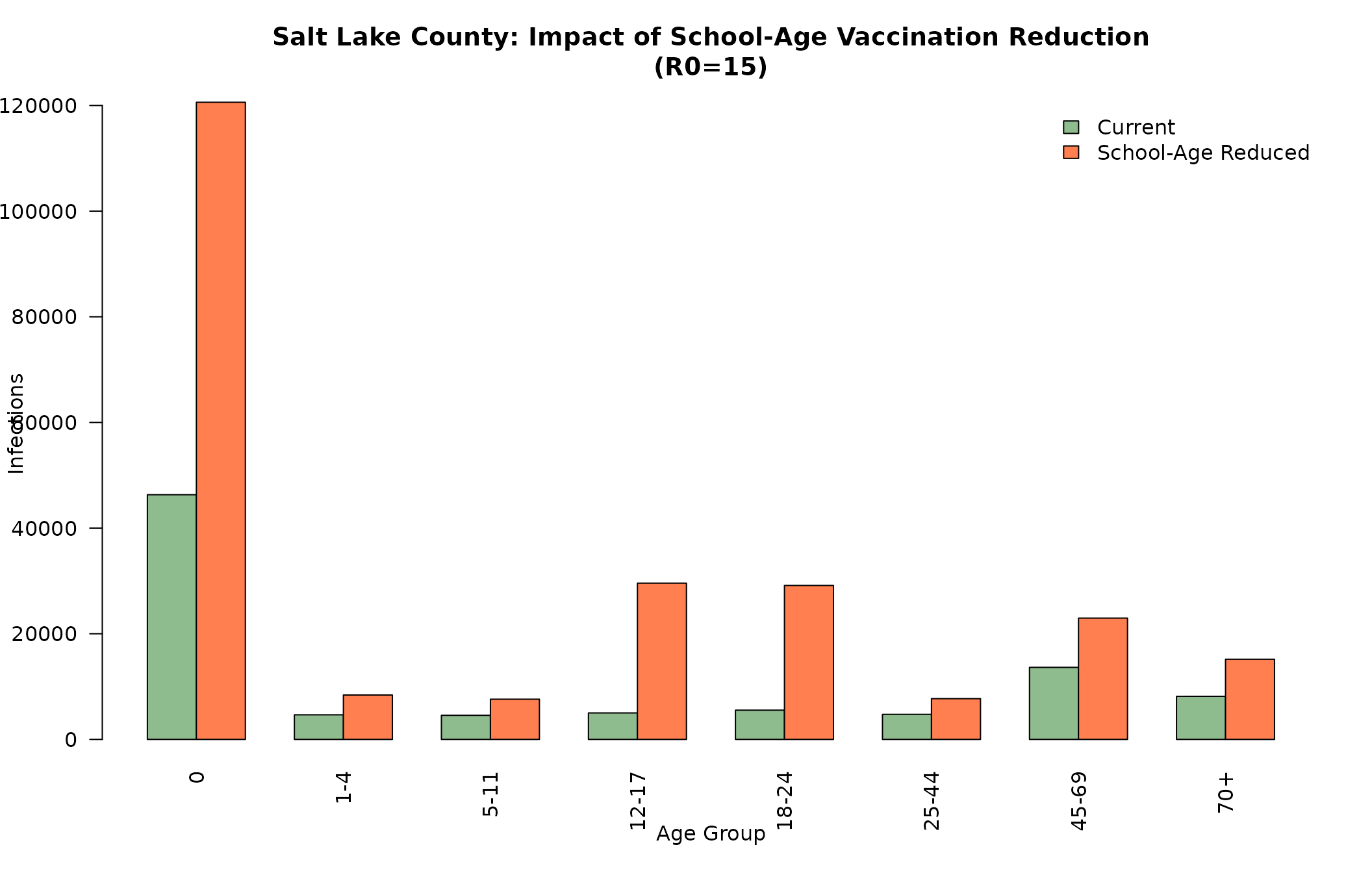
#> 25326 17556 0Age-Specific Impact
# Compare infections by age group for Salt Lake County
age_labels_short <- c("0", "1-4", "5-11", "12-17", "18-24", "25-44", "45-69", "70+")

# Get age-specific infections for R0=15
slc_current_ages <- as.numeric(slc_current[r0_15_idx, 5:12])
slc_schoolgap_ages <- as.numeric(slc_schoolgap[r0_15_idx, 5:12])

age_comparison <- rbind(slc_current_ages, slc_schoolgap_ages)
colnames(age_comparison) <- age_labels_short
rownames(age_comparison) <- c("Current", "School-Age Reduced")

barplot(age_comparison,
        beside = TRUE,
        main = "Salt Lake County: Impact of School-Age Vaccination Reduction\n(R0=15)",
        xlab = "Age Group",
        ylab = "Infections",
        col = c("darkseagreen", "coral"),
        legend.text = rownames(age_comparison),
        args.legend = list(x = "topright", bty = "n"),
        las = 2)