The data in this example in files named .demo.txt. Your own analysis should omit the .demo.
Admissions Data Overview
Admissions data shows all the admission to the facility in the entire run, as well as whether or not the patient admitted imported the disease.
WarningWarning:
After some iterations of the simulation, the last row of data in this file is not complete. If you see errors when you read in the data, check the .txt file and, if necessary, delete the last record.
# Read admissions.txt and show descriptive info and stats# Read admissions.txtadmissions_df <-read.table('../data/admissions.demo.txt', header=TRUE, sep=',', stringsAsFactors=FALSE)# Show structure cat('Admissions data:')
This dataset shows the time and patient id of a detection via the clinical (symptoms-base) route. DetectionCount is a check column. In some edge cases a patient may be detected, treated, recovered and detected again, in which case detection count for that patient would be >1.
#read clinical_detections and give descriptive stats.clinical_detections_df <-read.table('../data/clinicalDetection.demo.txt', header=TRUE, sep=',', stringsAsFactors=FALSE)#show sample of rows:head(clinical_detections_df)
      Time         DetectedPatientID DetectionCount
 Min.   :  26.83   Min.   :  107     Min.   :1
 1st Qu.:1388.93   1st Qu.: 4909     1st Qu.:1
 Median :2651.58   Median : 9331     Median :1
 Mean   :2695.46   Mean   : 9516     Mean   :1
 3rd Qu.:4014.90   3rd Qu.:14249     3rd Qu.:1
 Max.   :5467.43   Max.   :19151     Max.   :1
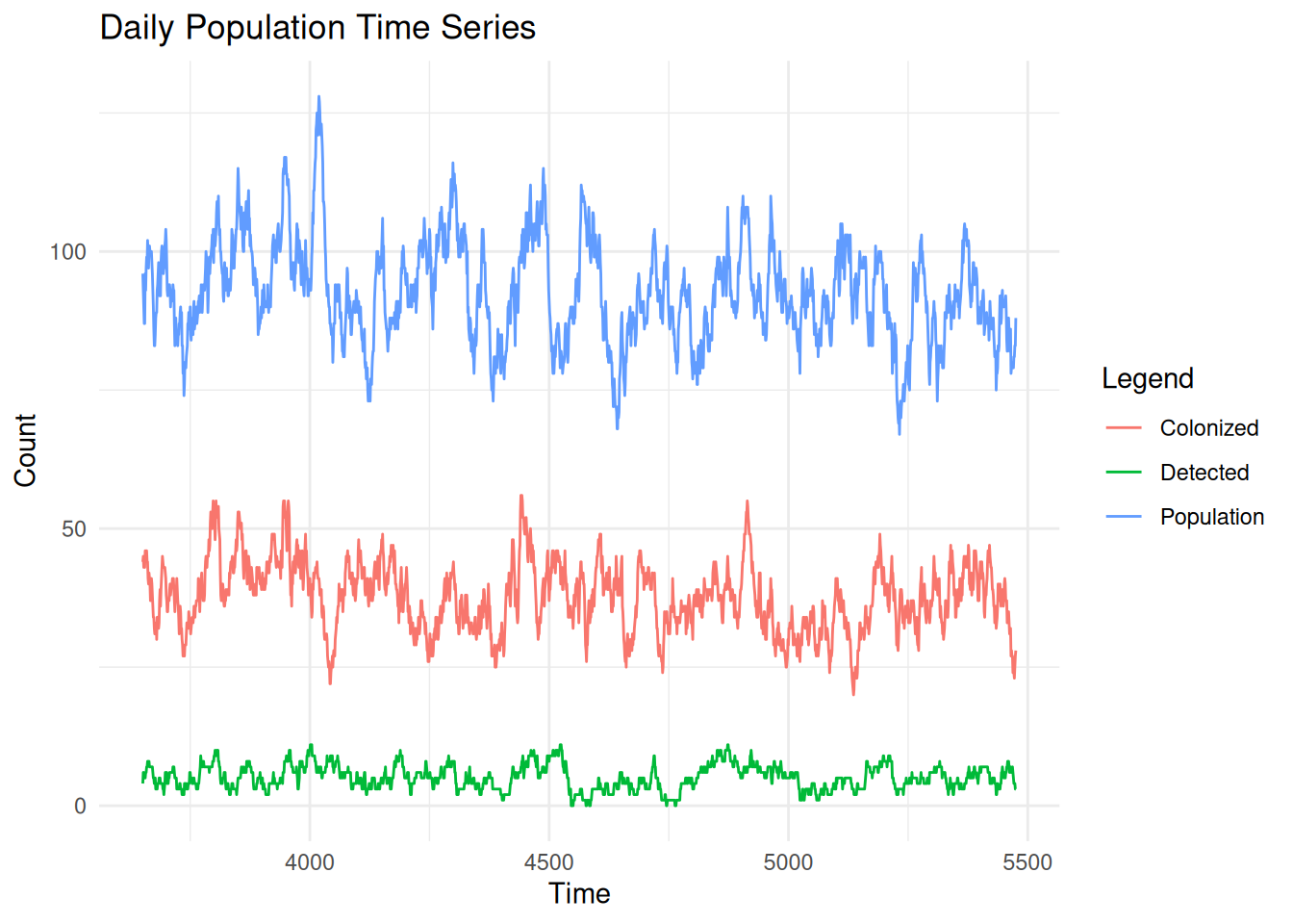
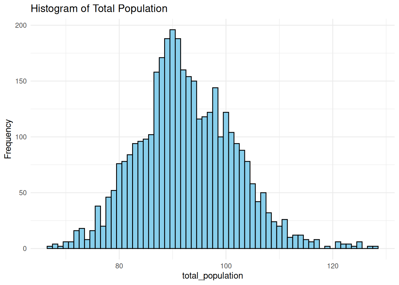
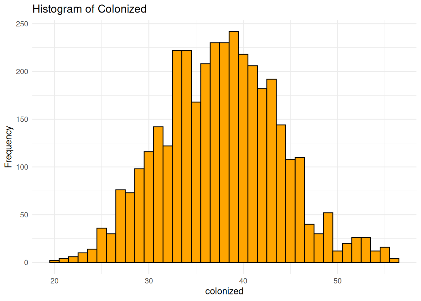
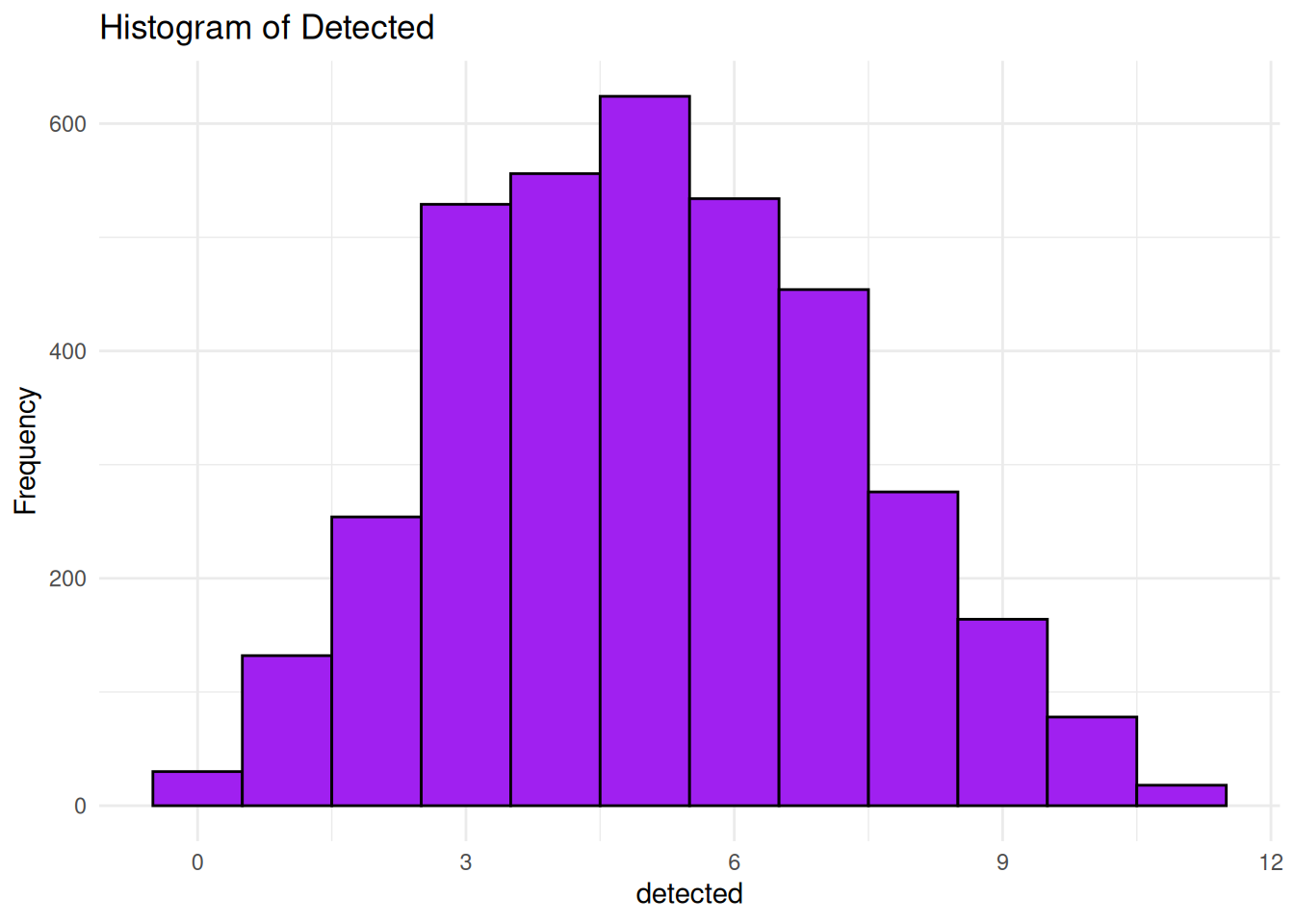
Daily Population Counts
The output file daily_population_stats.txt shows the total number of patients in the facility on a given day, the number of those who are colonized, detected and isolation. By default, it starts at the end of the burn-in period. There is another sanity check embedded in this file; it should always be the case that detected == isolated. We isolate detected patients, and we don’t isolate anybody else.
# Read daily_population_stats.txt (comma-delimited)daily_pop_df <-read.table('../data/daily_population_stats.demo.txt', header=TRUE, sep=',', stringsAsFactors=FALSE)# Show structure and summarycat('Daily population stats:')
      Time      total_population   colonized        detected
 Min.   :3651   Min.   : 67.00   Min.   :20.00   Min.   : 0.000
 1st Qu.:4107   1st Qu.: 87.00   1st Qu.:33.00   1st Qu.: 3.000
 Median :4563   Median : 92.00   Median :38.00   Median : 5.000
 Mean   :4563   Mean   : 92.63   Mean   :37.67   Mean   : 5.101
 3rd Qu.:5019   3rd Qu.: 99.00   3rd Qu.:42.00   3rd Qu.: 7.000
 Max.   :5475   Max.   :128.00   Max.   :56.00   Max.   :11.000
    isolated
 Min.   : 0.000
 1st Qu.: 3.000
 Median : 5.000
 Mean   : 5.101
 3rd Qu.: 7.000
 Max.   :11.000
Daily Population Time Series
# Time-series plot: population, colonized, detected vs timelibrary(ggplot2)# Assume columns: Time, total_population, colonized, detectedggplot(daily_pop_df, aes(x = Time)) +geom_line(aes(y =`total_population`, color ='Population')) +geom_line(aes(y = colonized, color ='Colonized')) +geom_line(aes(y = detected, color ='Detected')) +labs(title ='Daily Population Time Series', x ='Time', y ='Count', color ='Legend') +theme_minimal()
Distribution of Daily Population Values
These are the distribution of daily samples of the total population of the sim, the colonized and detected counts.
# Histogram of Total Populationggplot(daily_pop_df, aes(x = total_population)) +geom_histogram(binwidth =1, fill ='skyblue', color ='black') +labs(title ='Histogram of Total Population', x ='total_population', y ='Frequency') +theme_minimal()
# Histogram of Colonizedggplot(daily_pop_df, aes(x = colonized)) +geom_histogram(binwidth =1, fill ='orange', color ='black') +labs(title ='Histogram of Colonized', x ='colonized', y ='Frequency') +theme_minimal()
# Histogram of Detectedggplot(daily_pop_df, aes(x = detected)) +geom_histogram(binwidth =1, fill ='purple', color ='black') +labs(title ='Histogram of Detected', x ='detected', y ='Frequency') +theme_minimal()
Decolonization Events
These represent patients who’s colonization with the organism has ceased.
# Read decolonization.demo.txt (comma-delimited)decolonization_df <-read.table('../data/decolonization.demo.txt', header=TRUE, sep=',', stringsAsFactors=FALSE)# Show structure and summarycat('Decolonization events:')
      time         decolonized_patient_id
 Min.   :  23.89   Min.   :   75
 1st Qu.:1475.74   1st Qu.: 5145
 Median :2817.95   Median : 9883
 Mean   :2775.86   Mean   : 9751
 3rd Qu.:4091.78   3rd Qu.:14463
 Max.   :5470.71   Max.   :19207
Detection Verification Events
# Read detection_verification.demo.txt (comma-delimited)detection_verification_df <-read.table('../data/detection_verification.demo.txt', header=TRUE, sep=',', stringsAsFactors=TRUE)# Show structure and summarycat('Detection verification events:')
      time           patient_id         source     colonized   detection_count
 Min.   :  26.83   Min.   :  107   CLINICAL:1541   true:1541   Min.   :1
 1st Qu.:1388.93   1st Qu.: 4909                               1st Qu.:1
 Median :2651.58   Median : 9331                               Median :1
 Mean   :2695.46   Mean   : 9516                               Mean   :1
 3rd Qu.:4014.90   3rd Qu.:14249                               3rd Qu.:1
 Max.   :5467.43   Max.   :19151                               Max.   :1
Surveillance Events
This is every surveillance test run after the end of the burn-in period.
# Read surveillance.demo.txt (comma-delimited)# Check if file exists and has dataif (file.size('../data/surveillance.demo.txt') >0) { surveillance_df <-read.table('../data/surveillance.demo.txt', header=TRUE, sep=',', stringsAsFactors=FALSE)# Show structure and summarycat('Surveillance events:')head(surveillance_df)cat('\nSummary statistics:')summary(surveillance_df)} else {cat('No surveillance events in this dataset.\n')}