Batch Iteration Data Analysis

library(dplyr)

Attaching package: 'dplyr'
The following objects are masked from 'package:stats':

    filter, lag
The following objects are masked from 'package:base':

    intersect, setdiff, setequal, union
library(readr)
library(ggplot2)

# Read in the simulation outputs
sim_outputs <- read_csv("../data/sim_modeloutputs.demo.txt")
Rows: 404 Columns: 10
── Column specification ────────────────────────────────────────────────────────
Delimiter: ","
dbl (9): run, IsolationEffectiveness, DaysBetweenTests, tick, ClinicalDetect...
lgl (1): DoActiveSurveillance

ℹ Use `spec()` to retrieve the full column specification for this data.
ℹ Specify the column types or set `show_col_types = FALSE` to quiet this message.
# Read in the batch parameter map
batch_params <- read_csv("../data/sim_modeloutputs.batch_param_map.demo.txt")
Rows: 404 Columns: 25
── Column specification ────────────────────────────────────────────────────────
Delimiter: ","
chr  (1): diseaseName
dbl (19): run, isolationEffectiveness, shape1, shape2, importationRate, beta...
lgl  (5): allowImportationsDuringBurnIn, isBatchRun, isolatePatientWhenDetec...

ℹ Use `spec()` to retrieve the full column specification for this data.
ℹ Specify the column types or set `show_col_types = FALSE` to quiet this message.
# Join the datasets on the "run" column
combined_data <- sim_outputs %>%
  left_join(batch_params, by = "run")

# View the structure of the combined data
glimpse(combined_data)
Rows: 404
Columns: 34
$ run                             <dbl> 1, 19, 37, 55, 73, 91, 109, 127, 145, …
$ DoActiveSurveillance            <lgl> FALSE, FALSE, FALSE, FALSE, FALSE, FAL…
$ IsolationEffectiveness          <dbl> 0.5, 0.5, 0.5, 0.5, 0.5, 0.5, 0.5, 0.5…
$ DaysBetweenTests                <dbl> 7, 7, 7, 7, 7, 7, 7, 7, 7, 7, 7, 7, 7,…
$ tick                            <dbl> 5474, 5474, 5474, 5474, 5474, 5474, 54…
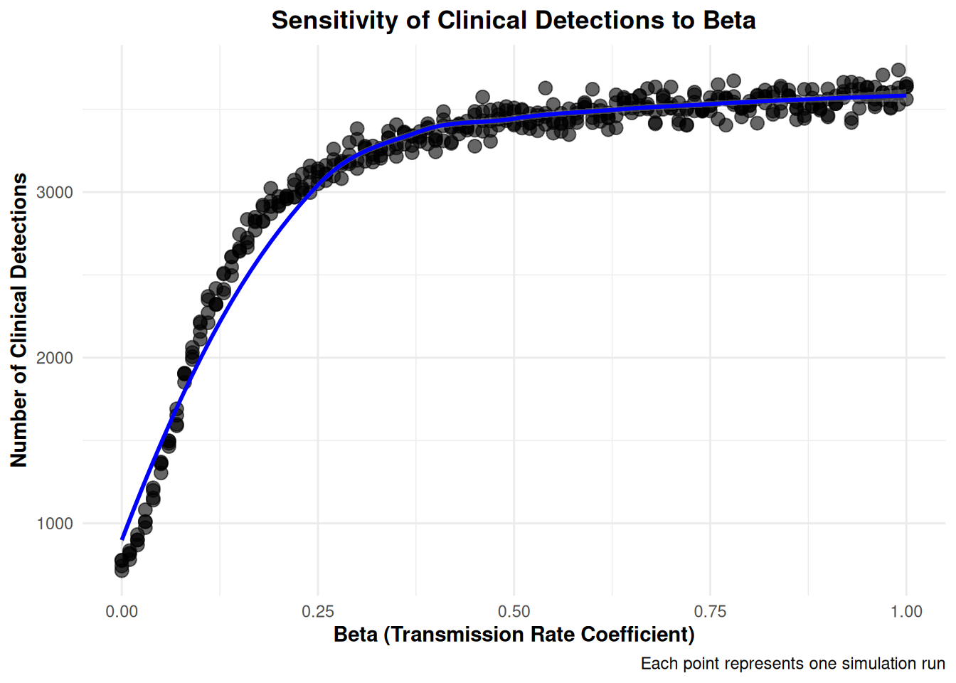
$ ClinicalDetections              <dbl> 777, 2922, 3358, 3408, 3498, 3623, 158…
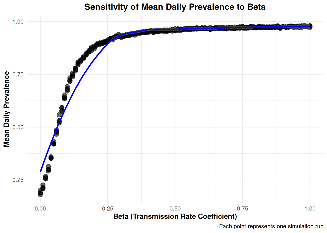
$ MeanDailyPrevalence             <dbl> 0.1801766, 0.8621268, 0.9486873, 0.965…
$ MeanDischargePrevalence         <dbl> 0.1943099, 0.8664326, 0.9491032, 0.969…
$ ImportationPrevalence           <dbl> 0.2090799, 0.2095499, 0.2051085, 0.210…
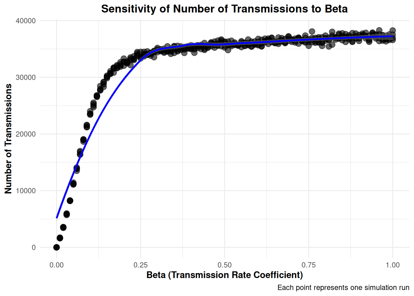
$ NumberOfTransmissions           <dbl> 0, 32138, 34586, 35672, 36904, 36422, …
$ allowImportationsDuringBurnIn   <lgl> FALSE, FALSE, FALSE, FALSE, FALSE, FAL…
$ isBatchRun                      <lgl> FALSE, FALSE, FALSE, FALSE, FALSE, FAL…
$ isolatePatientWhenDetected      <lgl> TRUE, TRUE, TRUE, TRUE, TRUE, TRUE, TR…
$ doActiveSurveillanceAfterBurnIn <lgl> FALSE, FALSE, FALSE, FALSE, FALSE, FAL…
$ isolationEffectiveness          <dbl> 0.5, 0.5, 0.5, 0.5, 0.5, 0.5, 0.5, 0.5…
$ diseaseName                     <chr> "CRE", "CRE", "CRE", "CRE", "CRE", "CR…
$ shape1                          <dbl> 7.60197, 7.60197, 7.60197, 7.60197, 7.…
$ shape2                          <dbl> 1.23279, 1.23279, 1.23279, 1.23279, 1.…
$ importationRate                 <dbl> 0.206, 0.206, 0.206, 0.206, 0.206, 0.2…
$ isActiveSurveillanceAgent       <lgl> TRUE, TRUE, TRUE, TRUE, TRUE, TRUE, TR…
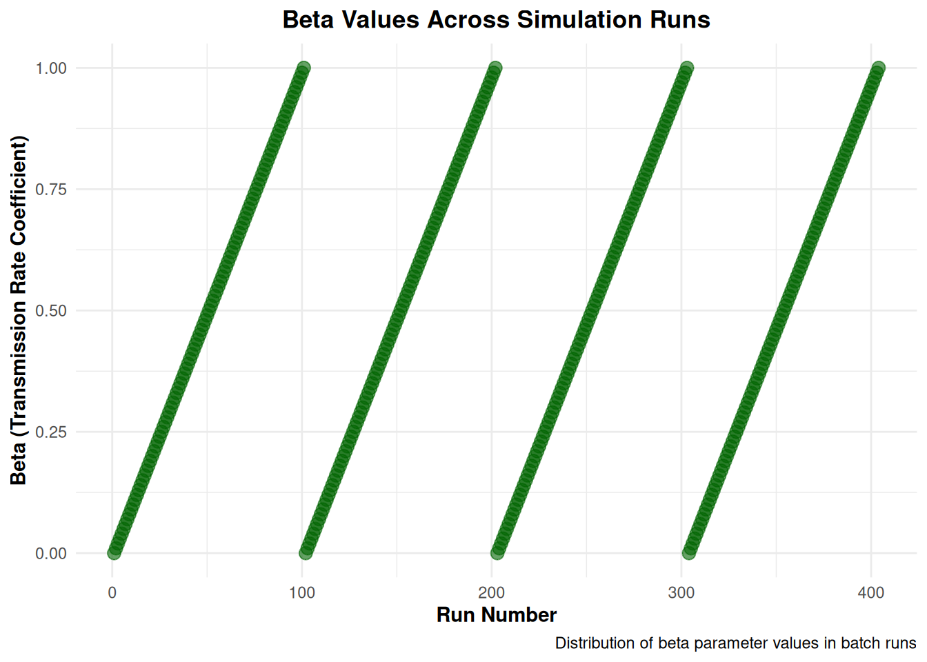
$ beta                            <dbl> 0.00, 0.18, 0.36, 0.54, 0.72, 0.90, 0.…
$ extraIteration                  <dbl> 1, 1, 1, 1, 1, 1, 2, 2, 2, 2, 2, 2, 3,…
$ prob1                           <dbl> 0.62531, 0.62531, 0.62531, 0.62531, 0.…
$ midstaySurveillanceAdherence    <dbl> 0.954, 0.954, 0.954, 0.954, 0.954, 0.9…
$ daysBetweenTests                <dbl> 7, 7, 7, 7, 7, 7, 7, 7, 7, 7, 7, 7, 7,…
$ simulationDurationAfterBurnIn   <dbl> 5475, 5475, 5475, 5475, 5475, 5475, 54…
$ randomSeed                      <dbl> -929615374, -929609984, -929571943, -9…
$ admissionSurveillanceAdherence  <dbl> 0.911, 0.911, 0.911, 0.911, 0.911, 0.9…
$ meanDetectionTime               <dbl> 122, 122, 122, 122, 122, 122, 122, 122…
$ avgDecolonizationTime           <dbl> 387, 387, 387, 387, 387, 387, 387, 387…
$ scale2                          <dbl> 23.52147, 23.52147, 23.52147, 23.52147…
$ scale1                          <dbl> 3.41952, 3.41952, 3.41952, 3.41952, 3.…
$ probSurveillanceDetection       <dbl> 0.8, 0.8, 0.8, 0.8, 0.8, 0.8, 0.8, 0.8…
$ burnInPeriod                    <dbl> 3650, 3650, 3650, 3650, 3650, 3650, 36…

Beta Parameter Distribution Across Runs

# Create scatter plot showing beta values across runs
ggplot(combined_data, aes(x = run, y = beta)) +
  geom_point(alpha = 0.6, size = 3, color = "darkgreen") +
  labs(
    title = "Beta Values Across Simulation Runs",
    x = "Run Number",
    y = "Beta (Transmission Rate Coefficient)",
    caption = "Distribution of beta parameter values in batch runs"
  ) +
  theme_minimal() +
  theme(
    plot.title = element_text(hjust = 0.5, face = "bold"),
    axis.title = element_text(face = "bold")
  )

Sensitivity Analysis: Beta vs Number of Transmissions

library(ggplot2)

# Create scatter plot showing beta sensitivity
ggplot(combined_data, aes(x = beta, y = NumberOfTransmissions)) +
  geom_point(alpha = 0.6, size = 3) +
  geom_smooth(method = "loess", se = TRUE, color = "blue") +
  labs(
    title = "Sensitivity of Number of Transmissions to Beta",
    x = "Beta (Transmission Rate Coefficient)",
    y = "Number of Transmissions",
    caption = "Each point represents one simulation run"
  ) +
  theme_minimal() +
  theme(
    plot.title = element_text(hjust = 0.5, face = "bold"),
    axis.title = element_text(face = "bold")
  )
`geom_smooth()` using formula = 'y ~ x'

Sensitivity Analysis: Beta vs Clinical Detections

# Create scatter plot showing beta sensitivity for clinical detections
ggplot(combined_data, aes(x = beta, y = ClinicalDetections)) +
  geom_point(alpha = 0.6, size = 3) +
  geom_smooth(method = "loess", se = TRUE, color = "blue") +
  labs(
    title = "Sensitivity of Clinical Detections to Beta",
    x = "Beta (Transmission Rate Coefficient)",
    y = "Number of Clinical Detections",
    caption = "Each point represents one simulation run"
  ) +
  theme_minimal() +
  theme(
    plot.title = element_text(hjust = 0.5, face = "bold"),
    axis.title = element_text(face = "bold")
  )
`geom_smooth()` using formula = 'y ~ x'

Sensitivity Analysis: Beta vs Mean Daily Prevalence

# Create scatter plot showing beta sensitivity for mean daily prevalence
ggplot(combined_data, aes(x = beta, y = MeanDailyPrevalence)) +
  geom_point(alpha = 0.6, size = 3) +
  geom_smooth(method = "loess", se = TRUE, color = "blue") +
  labs(
    title = "Sensitivity of Mean Daily Prevalence to Beta",
    x = "Beta (Transmission Rate Coefficient)",
    y = "Mean Daily Prevalence",
    caption = "Each point represents one simulation run"
  ) +
  theme_minimal() +
  theme(
    plot.title = element_text(hjust = 0.5, face = "bold"),
    axis.title = element_text(face = "bold")
  )
`geom_smooth()` using formula = 'y ~ x'

Sensitivity Analysis: Beta vs Mean Discharge Prevalence

# Create scatter plot showing beta sensitivity for mean discharge prevalence
ggplot(combined_data, aes(x = beta, y = MeanDischargePrevalence)) +
  geom_point(alpha = 0.6, size = 3) +
  geom_smooth(method = "loess", se = TRUE, color = "blue") +
  labs(
    title = "Sensitivity of Mean Discharge Prevalence to Beta",
    x = "Beta (Transmission Rate Coefficient)",
    y = "Mean Discharge Prevalence",
    caption = "Each point represents one simulation run"
  ) +
  theme_minimal() +
  theme(
    plot.title = element_text(hjust = 0.5, face = "bold"),
    axis.title = element_text(face = "bold")
  )
`geom_smooth()` using formula = 'y ~ x'