The data in this example in files named .demo.txt. Your own analysis should omit the .demo.
Admissions Data Overview
Admissions data shows all the admission to the facility in the entire run, as well as whether or not the patient admitted imported the disease.
WarningWarning:
After some iterations of the simulation, the last row of data in this file is not complete. If you see errors when you read in the data, check the .txt file and, if necessary, delete the last record.
# Read admissions.txt and show descriptive info and stats# Read admissions.txtadmissions_df <-read.table('../data/admissions.demo.txt', header=TRUE, sep=',', stringsAsFactors=FALSE)# Show structure cat('Admissions data:')
This dataset shows the time and patient id of a detection via the clinical (symptoms-base) route. DetectionCount is a check column. In some edge cases a patient may be detected, treated, recovered and detected again, in which case detection count for that patient would be >1.
#read clinical_detections and give descriptive stats.clinical_detections_df <-read.table('../data/clinicalDetection.demo.txt', header=TRUE, sep=',', stringsAsFactors=FALSE)#show sample of rows:head(clinical_detections_df)
      Time         DetectedPatientID DetectionCount
 Min.   :   2.66   Min.   :   83     Min.   :1
 1st Qu.:1038.26   1st Qu.: 3795     1st Qu.:1
 Median :2262.56   Median : 8179     Median :1
 Mean   :2363.93   Mean   : 8462     Mean   :1
 3rd Qu.:3457.09   3rd Qu.:12349     3rd Qu.:1
 Max.   :5464.87   Max.   :19628     Max.   :1
Daily Population Counts
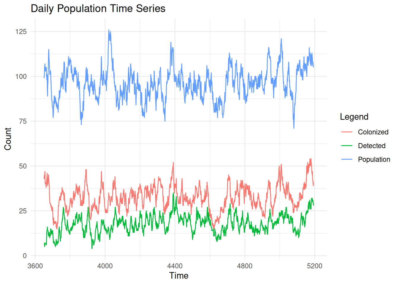
The output file daily_population_stats.txt shows the total number of patients in the facility on a given day, the number of those who are colonized, detected and isolation. By default, it starts at the end of the burn-in period. There is another sanity check embedded in this file; it should always be the case that detected == isolated. We isolate detected patients, and we don’t isolate anybody else.
# Read daily_population_stats.txt (comma-delimited)daily_pop_df <-read.table('../data/daily_population_stats.demo.txt', header=TRUE, sep=',', stringsAsFactors=FALSE)# Show structure and summarycat('Daily population stats:')
      time      total_population   colonized        detected
 Min.   :3651   Min.   : 71.0    Min.   :15.00   Min.   : 4.00
 1st Qu.:4036   1st Qu.: 90.0    1st Qu.:28.00   1st Qu.:14.00
 Median :4422   Median : 96.0    Median :32.00   Median :18.00
 Mean   :4422   Mean   : 96.2    Mean   :32.68   Mean   :17.64
 3rd Qu.:4807   3rd Qu.:102.0    3rd Qu.:38.00   3rd Qu.:21.00
 Max.   :5193   Max.   :126.0    Max.   :54.00   Max.   :35.00
    isolated
 Min.   : 4.00
 1st Qu.:14.00
 Median :18.00
 Mean   :17.64
 3rd Qu.:21.00
 Max.   :35.00
Daily Population Time Series
# Time-series plot: population, colonized, detected vs timelibrary(ggplot2)# Assume columns: time, Total Population, Colonized, Detectedggplot(daily_pop_df, aes(x = time)) +geom_line(aes(y =`total_population`, color ='Population')) +geom_line(aes(y = colonized, color ='Colonized')) +geom_line(aes(y = detected, color ='Detected')) +labs(title ='Daily Population Time Series', x ='Time', y ='Count', color ='Legend') +theme_minimal()
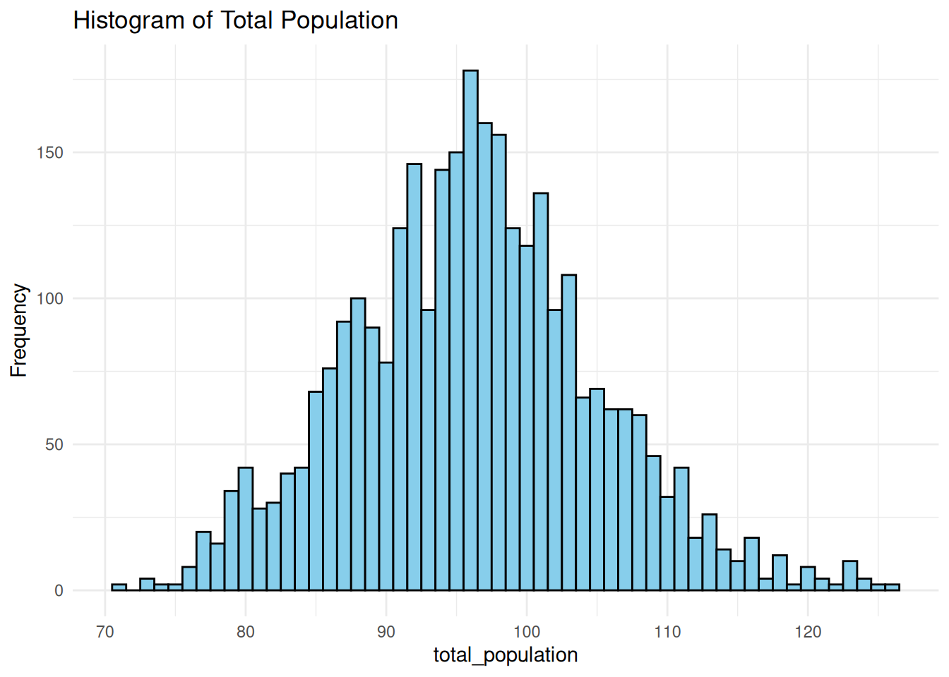
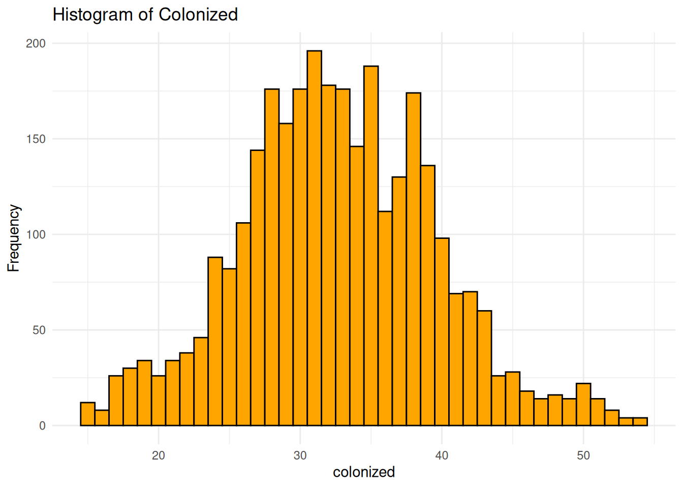
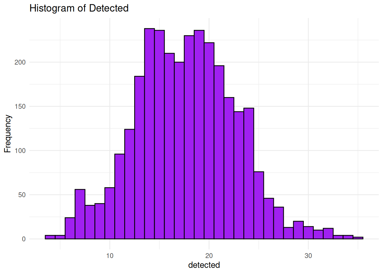
Distribution of Daily Population Values
These are the distribution of daily samples of the total population of the sim, the colonized and detected counts.
# Histogram of Total Populationggplot(daily_pop_df, aes(x = total_population)) +geom_histogram(binwidth =1, fill ='skyblue', color ='black') +labs(title ='Histogram of Total Population', x ='total_population', y ='Frequency') +theme_minimal()
# Histogram of Colonizedggplot(daily_pop_df, aes(x = colonized)) +geom_histogram(binwidth =1, fill ='orange', color ='black') +labs(title ='Histogram of Colonized', x ='colonized', y ='Frequency') +theme_minimal()
# Histogram of Detectedggplot(daily_pop_df, aes(x = detected)) +geom_histogram(binwidth =1, fill ='purple', color ='black') +labs(title ='Histogram of Detected', x ='detected', y ='Frequency') +theme_minimal()
Decolonization Events
These represent patients who’s colonization with the organism has ceased.
# Read decolonization.demo.txt (comma-delimited)decolonization_df <-read.table('../data/decolonization.demo.txt', header=TRUE, sep=',', stringsAsFactors=FALSE)# Show structure and summarycat('Decolonization events:')
      time         decolonized_patient_id
 Min.   :  14.72   Min.   :   78
 1st Qu.:1307.01   1st Qu.: 4530
 Median :2695.80   Median : 9473
 Mean   :2654.49   Mean   : 9431
 3rd Qu.:3913.38   3rd Qu.:13925
 Max.   :5465.38   Max.   :19624
Detection Verification Events
# Read detection_verification.demo.txt (comma-delimited)detection_verification_df <-read.table('../data/detection_verification.demo.txt', header=TRUE, sep=',', stringsAsFactors=TRUE)# Show structure and summarycat('Detection verification events:')
      time           patient_id             source     colonized
 Min.   :  10.12   Min.   :   79   CLINICAL    :1266   true:2913
 1st Qu.:2673.47   1st Qu.: 9480   SURVEILLANCE:1647
 Median :4056.75   Median :14263
 Mean   :3622.80   Mean   :12767
 3rd Qu.:4791.95   3rd Qu.:16841
 Max.   :5474.36   Max.   :19347
 detection_count
 Min.   :0.0000
 1st Qu.:0.0000
 Median :0.0000
 Mean   :0.4346
 3rd Qu.:1.0000
 Max.   :1.0000
Surveillance Events
This is every surveillance test run after the end of the burn-in period.
# Read surveillance.demo.txt (comma-delimited)surveillance_df <-read.table('../data/surveillance.demo.txt', header=TRUE, sep=',', stringsAsFactors=FALSE)# Show structure and summarycat('Surveillance events:')
      Time         Patient       Colonized           Detected
 Min.   :3664   Min.   :13233   Length:7106        Length:7106
 1st Qu.:4081   1st Qu.:14701   Class :character   Class :character
 Median :4481   Median :16148   Mode  :character   Mode  :character
 Mean   :4491   Mean   :16163
 3rd Qu.:4901   3rd Qu.:17614
 Max.   :5335   Max.   :19150
      time         from_patientID   to_patientID
 Min.   :   6.45   Min.   :   75   Min.   :   75
 1st Qu.:1140.95   1st Qu.: 4021   1st Qu.: 4028
 Median :2273.90   Median : 8083   Median : 8114
 Mean   :2311.97   Mean   : 8157   Mean   : 8173
 3rd Qu.:3452.97   3rd Qu.:12165   3rd Qu.:12152
 Max.   :4881.69   Max.   :17098   Max.   :17166
                                   NA's   :1