Part 3: Mixing Models

Note

This example has been adapted from the ongoing work on the FIFA World Cup, InsightNet’s ID Cup https://github.com/EpiForeSITE/idcup.

Now, we will build a more complex model using the ModelSEIRMixingQuarantine() model. The new model has the following components:

• Contact Matrix: Using data from Epistorm (Litvinova et al. 2025), this provides a contact matrix at the group level, indicating the average number of contacts between age groups.
• Heterogenous Vaccination: We can specify vaccination rates to be heterogenous at the group level.
• Contact tracing and isolation: This is built-in feature in the model. Although users could implement their own using R, it is not recommended as the C++ version is highly efficient.

Preparing the environment

library(epiworldR)
library(measles)
library(data.table)
library(ggplot2)

params <- list(
  city     = "Miami",
  max_pop  = 10000,
  nthreads = 4,
  seed     = 8812,
  ndays    = 60,
  nsims    = 100
)

Pulling information about the city and population from the data files. The mixing matrix is based on the EpiStorm (Litvinova et al. 2025) survey data, which provides age-based contact patterns for various cities. We will use the mixing matrix corresponding to the specified city in params$city.

# Population matrix
census_age <- fread("data/census_age.csv")[city == params$city]
population <- 487014

# Mixing matrix (age-based, from Epistorm survey data)
mixing_matrices <- readRDS("data/mixing_matrix.rds")

The total population in the census data 487014, exceeds the maximum population size (10000). The population will be scaled down to fit within the specified maximum population size.

N <- min(params$max_pop, sum(population))

census_age[, total := ceiling(total / sum(total) * N)]
N <- sum(census_age$total)

We calibrate the contact matrix to a target basic reproduction number of 2.5, consistent with a moderately transmissible respiratory pathogen (e.g., pandemic influenza). The infectious period is set to 7 days and the per-contact transmission probability to 0.1.

calib_scale <- calibrate_mixing_model(
  contact_matrix         = mixing_matrices,
  target_rep_number      = 2,
  infectious_period_days = 7,
  transmission_prob      = 0.1
)

Baseline scenario

# Hospitalization rate such that P(hosp) = 20%
# P(hosp) = hosp_r / (hosp_r + rec_r)
#   => hosp_r = P(hosp) * rec_r / (1 - P(hosp))
h_rate <- 0.2 * (1 / 7) / (1 - 0.2)

seir_model <- ModelSEIRMixingQuarantine(
  name                         = "Respiratory pathogen",
  n                            = N,
  prevalence                   = 10 / N,
  transmission_rate            = 0.1,
  incubation_days              = 5,
  recovery_rate                = 1 / 7,
  contact_matrix               = mixing_matrices * calib_scale,
  hospitalization_rate         = h_rate,
  hospitalization_period       = 7,
  # Detection and intervention parameters
  days_undetected              = 3,
  quarantine_period            = 7,
  quarantine_willingness       = 0.8,
  isolation_willingness        = 0.6,
  isolation_period             = 7,
  # Contact tracing parameters
  contact_tracing_success_rate = 0.5,
  contact_tracing_days_prior   = 4
)

# Adding age-group entities to the model
add_entities_from_dataframe(
  model        = seir_model,
  entities     = census_age,
  col_name     = "age_group",
  col_number   = "total",
  as_proportion = FALSE
)

We will use a single initial infectious case seeded randomly in the population.

get_virus(seir_model, 0L) |>
  set_distribution_virus(
    distfun = distribute_virus_randomly(
      prevalence    = 10,
      as_proportion = FALSE
    )
  )

We can now run the simulations.

saver <- make_saver("outbreak_size", "hospitalizations", "transition")

seir_model |>
  run_multiple(
    ndays    = params$ndays,
    nsims    = params$nsims,
    seed     = params$seed,
    saver    = saver,
    nthreads = 1 # params$nthreads
  )

Starting multiple runs (100) using 1 thread(s)
_________________________________________________________________________
_________________________________________________________________________
||||||||||||||||||||||||||||||||||||||||||||||||||||||||||||||||||||||||| done.

We can check the results of the simulations by summarizing the model:

summary(seir_model)

________________________________________________________________________________
________________________________________________________________________________
SIMULATION STUDY

Name of the model   : SEIR with Mixing and Quarantine
Population size     : 10009
Agents' data        : (none)
Number of entities  : 17
Days (duration)     : 60 (of 60)
Number of viruses   : 1
Last run elapsed t  : 0.00s
Total elapsed t     : 5.00s (100 runs)
Last run speed      : 10.84 million agents x day / second
Average run speed   : 11.92 million agents x day / second
Rewiring            : off
Last seed used      : 628712762

Global events:
 - Update infected individuals (runs daily)

Virus(es):
 - Respiratory pathogen

Tool(s):
 (none)

Model parameters:
 - Avg. Incubation days         : 5.0000
 - Contact tracing days prior   : 4.0000
 - Contact tracing success rate : 0.5000
 - Days undetected              : 3.0000
 - Hospitalization period       : 7.0000
 - Hospitalization rate         : 0.0357
 - Isolation period             : 7.0000
 - Isolation willingness        : 0.6000
 - Prob. Recovery               : 0.1429
 - Prob. Transmission           : 0.1000
 - Quarantine period            : 7.0000
 - Quarantine willingness       : 0.8000

Distribution of the population at time 60:
  - (0) Susceptible             :  9999 -> 9906
  - (1) Exposed                 :    10 -> 3
  - (2) Infected                :     0 -> 3
  - (3) Isolated                :     0 -> 5
  - (4) Quarantined Susceptible :     0 -> 30
  - (5) Quarantined Exposed     :     0 -> 3
  - (6) Isolated Recovered      :     0 -> 2
  - (7) Hospitalized            :     0 -> 5
  - (8) Recovered               :     0 -> 52

Transition Probabilities:
 - Susceptible              1.00  0.00     -     -  0.00  0.00     -     -     -
 - Exposed                     -  0.78  0.17     -     -  0.05     -     -     -
 - Infected                    -     -  0.73  0.09     -     -  0.02  0.06  0.10
 - Isolated                    -     -  0.09  0.71     -     -  0.13  0.05  0.02
 - Quarantined Susceptible  0.13     -     -     -  0.87     -     -     -     -
 - Quarantined Exposed         -  0.05     -  0.21     -  0.74     -     -     -
 - Isolated Recovered          -     -     -     -     -     -  0.70     -  0.30
 - Hospitalized                -     -     -     -     -     -     -  0.89  0.11
 - Recovered                   -     -     -     -     -     -     -     -  1.00

Extracting and plotting the results

ans <- seir_model |>
  run_multiple_get_results(
    freader = data.table::fread
  )

outbreak_size    <- ans$outbreak_size    |> as.data.table()
hospitalizations <- ans$hospitalizations |> as.data.table()
transition       <- ans$transition       |> as.data.table()

Transition

tmat <- get_transition_probability(seir_model) * 0

t_totals <- transition[, .(total = sum(counts)), by = .(from, to)]
tmat[as.matrix(t_totals[, .(from, to)])] <- t_totals$total

draw_mermaid_from_matrix(tmat) |>
  plot()

Outbreak size

ggplot(
  outbreak_size,
  aes(x = date, y = outbreak_size)
) +
  geom_point(
    color = "steelblue",
    alpha = 0.2,
    size  = 1.5
  ) +
  labs(
    title    = paste("SEIR outbreak size in", params$city),
    subtitle = sprintf(
      "Mixing model with census data (%i simulations)",
      params$nsims
    ),
    x = "Day",
    y = "Cases"
  ) +
  theme_minimal()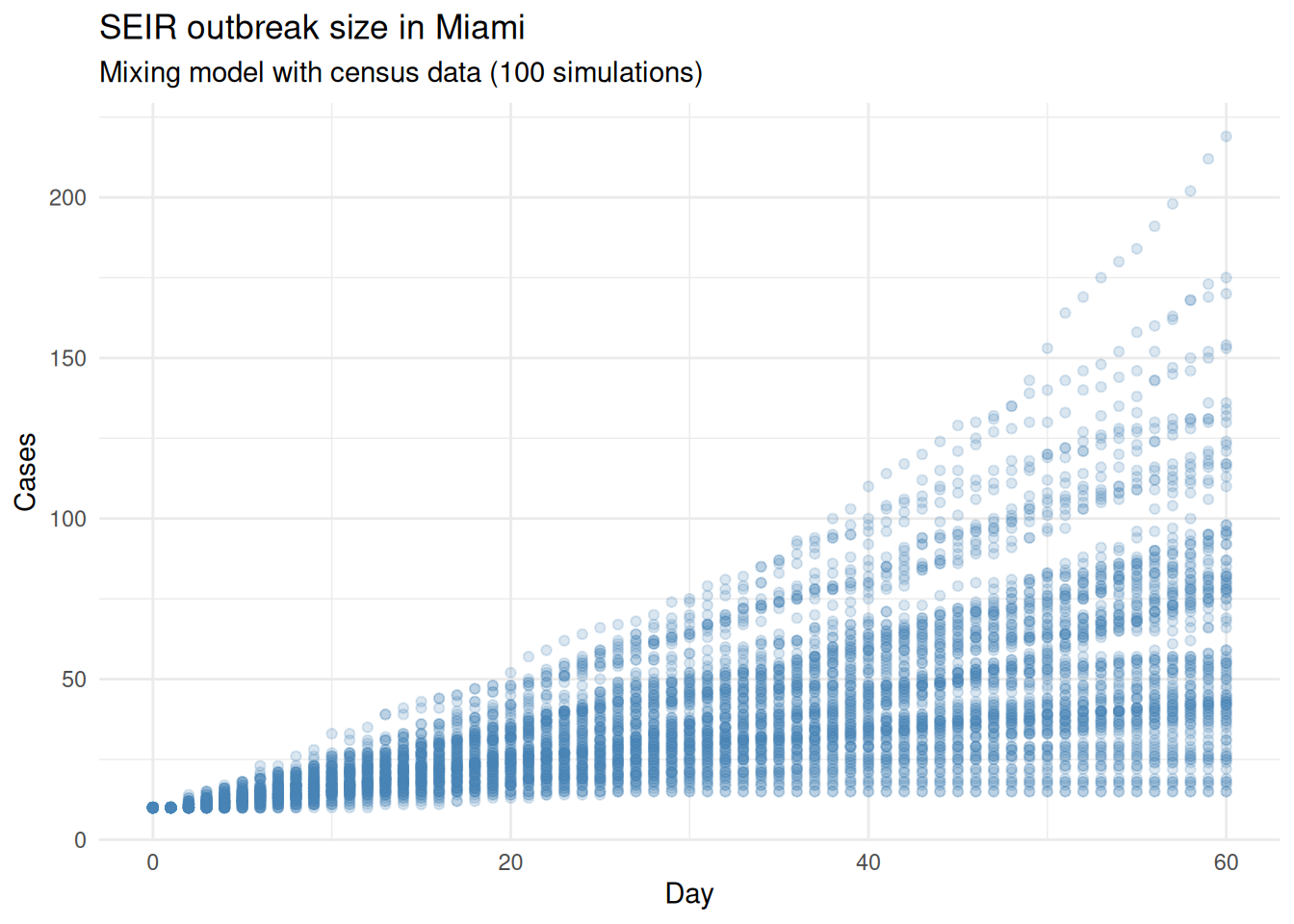

final_outbreak      <- outbreak_size[date == max(date)]
median_outbreak_size <- median(final_outbreak$outbreak_size)

ggplot(final_outbreak, aes(x = outbreak_size)) +
  geom_histogram(fill = "steelblue", color = "white") +
  labs(
    title    = sprintf(
      "SEIR outbreak size in %s (median: %.0f)",
      params$city,
      median_outbreak_size
    ),
    subtitle = sprintf(
      "Mixing model with census data (%i simulations)",
      params$nsims
    ),
    x = "Final outbreak size",
    y = "Count"
  ) +
  theme_minimal()

`stat_bin()` using `bins = 30`. Pick better value `binwidth`.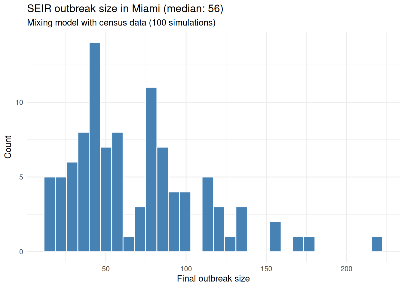

Hospitalizations

hosp_daily <- hospitalizations[, .(Total = sum(count)), by = .(sim_num)]

ggplot(hosp_daily, aes(x = Total)) +
  geom_histogram() +
  labs(
    title    = paste(
      "Daily hospitalizations in SEIR outbreak in",
      params$city
    ),
    subtitle = sprintf(
      "SEIR mixing model (%i simulations)",
      params$nsims
    ),
    y = "Frequency",
    x = "Total Hospitalizations"
  ) +
  theme_minimal()

`stat_bin()` using `bins = 30`. Pick better value `binwidth`.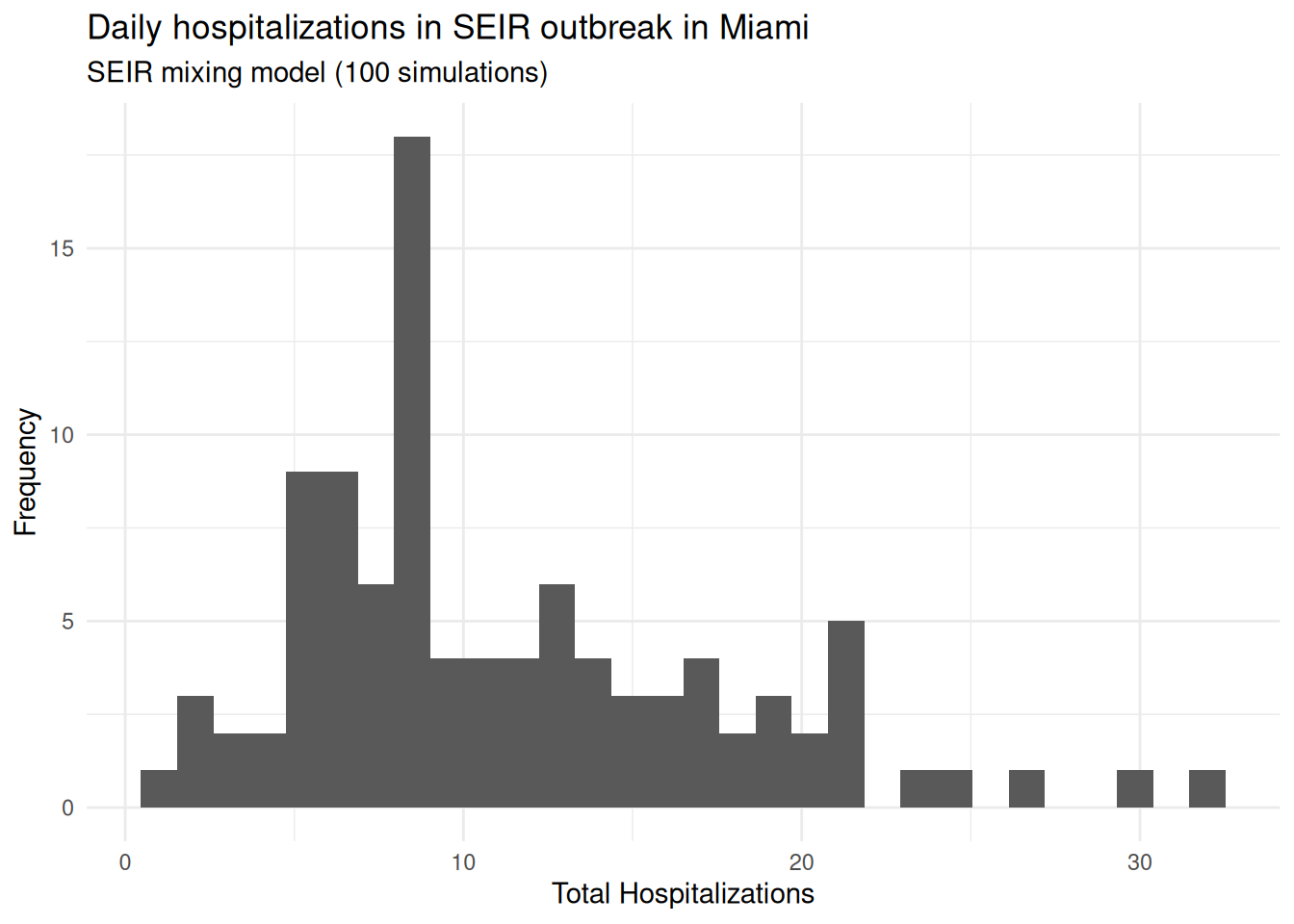

Intervention: reducing contact rates by 75%

Interventions in epiworldR can be applied in various forms. Besides changing the initial conditions, we can change the situation midway through the simulation using global events. Global events are functions that can arbitrarily modify the model at user-defined points in time. Some of the common applications are:

• globalevent_set_params(): Change model parameters (e.g., transmission rate, recovery rate, etc.) at a specific day.
• globalevent_tool(): Distribute a tool (e.g., vaccine, antiviral, etc.) to the population at a specific day.
• globalevent_fun(): Apply an arbitrary R function to the model at a specific day. This is the most flexible option, as it allows users to implement any intervention that can be coded in R. However, it is also the least efficient option, as it requires running the simulation in a single thread.

WarningThread safety

Unfortunately, the R programming language is not thread safe. In other words, when we use the globalevent_fun() caller, which essentially wraps an R function, we need to run the run_multiple() function using a single thread.

Global events can, as I mentioned, modify arbitrary parts of the program. In this case, we will use a global event to reduce the contact rates by 75% starting from day 40. This is equivalent to reducing the contact matrix by a factor of 4. To do so, we need two steps:

# Step 1: Create a R function that receives a model
reduce_contact_fourth <- function(m) {

  cmat <- epiworldR::get_contact_matrix(m)
  epiworldR::set_contact_matrix(
    m, cmat / 4,
    as_backup = FALSE
  )

}

# Step 2: Register (add) the event to the model
add_globalevent(
  model = seir_model,
  event = globalevent_fun(
    fun  = reduce_contact_fourth,
    name = "Reduce contact",
    day  = 40
    )
  )

The as_backup = FALSE tells epiworldR to automatically restore the original contact matrix when restarting the simulation. Let’s see how the model changes with this new event.

saver2 <- make_saver("outbreak_size")

seir_model |>
  run_multiple(
    ndays    = params$ndays,
    nsims    = params$nsims,
    seed     = params$seed,
    saver    = saver2,
    nthreads = 1 # params$nthreads
  )

Starting multiple runs (100) using 1 thread(s)
_________________________________________________________________________
_________________________________________________________________________
||||||||||||||||||||||||||||||||||||||||||||||||||||||||||||||||||||||||| done.

## Extracting
ans2 <- seir_model |>
  run_multiple_get_results(
    freader = data.table::fread
  )

outbreak_size2 <- ans2$outbreak_size |> as.data.table()

Now we can plot the result:

ggplot(
  outbreak_size2,
  aes(x = date, y = outbreak_size)
) +
  geom_point(
    color = "steelblue",
    alpha = 0.2,
    size  = 1.5
  ) +
  labs(
    title    = paste("SEIR outbreak size in", params$city),
    subtitle = sprintf(
      "Mixing model with census data (%i simulations)",
      params$nsims
    ),
    caption = "Includes intervention reducing contact rates",
    x = "Day",
    y = "Cases"
  ) +
  theme_minimal()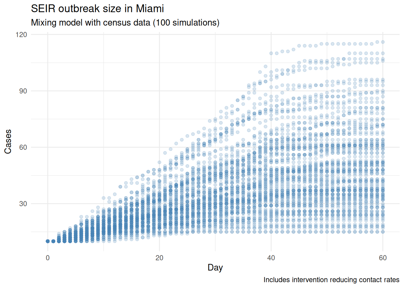

Exercises

1. Instead of using the glovalevent_fun(), let’s start a vaccination campaign in which we vaccinate 20% of the population on two separate days. Try to implement this intervention.

2. Using the parameter intervention, see if doubling the quarantine duration from its current value by day 30 has an effect.

3. (bonus) One advanced feature of epiworldR is the ability to add custom states and functions. Modify the infectious state to transition to recovered and deceased state (new state). Take a look at the model builder documentation.

Session info

This document was generated using the {epiworldR} package version 0.15.1.0 on 2026-04-29. We used R version 4.5.3, running on Linux with x86_64 architecture.

References

Litvinova, Maria, Shelly Sinclair, Allisandra G. Kummer, et al. 2025. Epistorm-Mix: Mapping Social Contact Patterns for Respiratory Pathogen Spread in the Post-Pandemic United States. medRxiv. https://doi.org/10.1101/2025.11.20.25340662.