Methodology

Published

December 18, 2025

source("functions.R")

Introduction

Here we provide details on our methodology for calibrating and running our forecast, as well as a description of the technologies powering the epiworld-forecasts tool.

Forecast Methodology

We use case count data published weekly by the Utah DHHS. The calibration and SIR connected model are run using the epiworldR package.

COVID-19 Cases in Utah (last 90 days)

Every week, Utah DHHS publishes COVID-19 surveillance data on their Coronavirus Dashboard which includes reported case counts for each day starting March 18, 2020. Our forecast is calibrated on case counts from the last 90 days.

# Define forecast parameters
n_days <- 90 # Calibrate model last 90 days of data

# Get COVID-19 data
covid_data <- get_covid_data(n_days)
plot_covid_data(covid_data)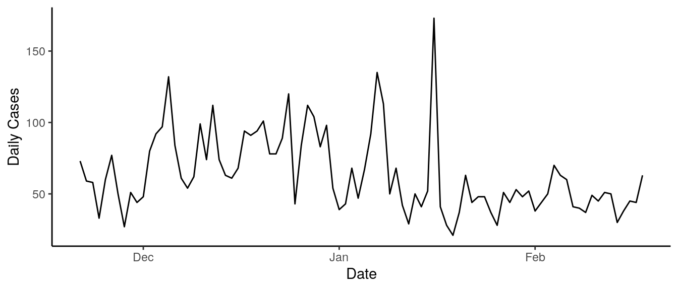

Calibrating the Forecasting Model

We use epiworldR’s implementation of Likelihood-Free Markhov Chain Monte Carlo (LFMCMC) to calibrate the SIR connected model (using ModelSIRCONN from epiworldR) by estimating the following model parameters:

Recovery rate
Transmission rates for each season (spring, summer, fall, winter)
Contact rates for weekdays and weekends

The LFMCMC simulation runs for 6,000 iterations. In each iteration, it does the following:

Proposes a new set of parameter values
Runs the model with 10,000 agents and the proposed parameters
Compares the output to the UDHHS data and records the result

We note that while the population of Utah over 3 million, we only need to run our model with 10,000 agents. This is because we don’t expect more than 10,000 COVID-19 cases and the model automatically scales the contact rate to account for the difference between the model population and Utah’s population.

COVID-19 Forecast

We start by preparing the model

# Compute start date for each season
seasons <- get_season_starts(covid_data$Date)

# Get observed case counts
covid_cases <- covid_data$Daily.Cases

# Define SIRCONN model parameters
model_seed          <- 112      # Random seed
model_ndays         <- n_days   # How many days to run the model
model_n             <- 10000    # model population size

# Define initial disease parameters
init_prevalence <- covid_cases[1] / model_n
init_contact_rate <- 20
init_transmission_rate <- 0.025
init_recovery_rate <- 1 / 7

# Create the SIRCONN model
covid_sirconn_model <- ModelSIRCONN(
  name              = "COVID-19",
  n                 = model_n,
  prevalence        = init_prevalence,
  contact_rate      = init_contact_rate,
  transmission_rate = init_transmission_rate,
  recovery_rate     = init_recovery_rate
)

We then continue setting the model parameters. The definition of the model itself is in the functions.R script.

# Define LFMCMC parameters
lfmcmc_n_samples <- 4000   # number of LFMCMC iterations
lfmcmc_burnin <- floor(lfmcmc_n_samples / 2)    # burn-in period
lfmcmc_epsilon <- 0.25

init_lfmcmc_params <- c(
  1 / 7,  # r_rate
  0.025,   # t_rate_spring
  0.02,   # t_rate_summer
  0.03,   # t_rate_fall
  0.035,   # t_rate_winter
  20,     # c_rate_weekday
  2       # c_rate_weekend
)
param_names <- c(
  "Recovery rate",
  "Transmission rate (spring)",
  "Transmission rate (summer)",
  "Transmission rate (fall)",
  "Transmission rate (winter)",
  "Contact rate (weekday)",
  "Contact rate (weekend)"
)

stats_names <- c(
  "Time to peak",
  "Size of peak",
  "Mean (cases)",
  "Standard deviation (cases)"
)

With all the needed components for the LFMCMC, we can now run the calibration.

# Create the LFMCMC object
calibration_lfmcmc <- LFMCMC(covid_sirconn_model) |>
  set_simulation_fun(lfmcmc_simulation_fun) |>
  set_summary_fun(lfmcmc_summary_fun) |>
  set_proposal_fun(lfmcmc_proposal_fun) |>
  set_kernel_fun(lfmcmc_kernel_fun) |>
  set_observed_data(covid_cases)

# Run LFMCMC calibration
run_lfmcmc(
  lfmcmc = calibration_lfmcmc,
  params_init = init_lfmcmc_params,
  n_samples = lfmcmc_n_samples,
  epsilon = lfmcmc_epsilon,
  seed = model_seed
)

_________________________________________________________________________
||||||||||||||||||||||||||||||||||||||||||||||||||||||||||||||||||||||||| done.

set_params_names(calibration_lfmcmc, param_names)
set_stats_names(calibration_lfmcmc, stats_names)

When the simulation is finished, we use a burn-in period of n = 2,000 (50% of simulation iterations). The epiworldR results printout (below) shows the mean parameter/statistic value, the 95% credible interval (in [ ]), and the initial/observed value (in ( )).

print(calibration_lfmcmc, burnin = lfmcmc_burnin)

___________________________________________

LIKELIHOOD-FREE MARKOV CHAIN MONTE CARLO

N Samples (total) : 4000
N Samples (after burn-in period) : 2000
Elapsed t : 3.00m

Parameters:
  -Recovery rate              :   0.33 [  0.26,   0.39] (initial :   0.14)
  -Transmission rate (spring) :   0.01 [  0.01,   0.02] (initial :   0.03)
  -Transmission rate (summer) :   0.03 [  0.02,   0.05] (initial :   0.02)
  -Transmission rate (fall)   :   0.09 [  0.06,   0.13] (initial :   0.03)
  -Transmission rate (winter) :   0.03 [  0.03,   0.04] (initial :   0.04)
  -Contact rate (weekday)     :  19.46 [ 18.68,  20.19] (initial :  20.00)
  -Contact rate (weekend)     :   0.64 [  0.25,   0.95] (initial :   2.00)

Statistics:
  -Time to peak               :   21.12 [   1.00,   22.00] (Observed:   19.00)
  -Size of peak               :  137.33 [  60.00,  198.00] (Observed:  162.00)
  -Mean (cases)               :   15.04 [   7.21,   26.56] (Observed:   38.78)
  -Standard deviation (cases) :   28.38 [  13.94,   41.10] (Observed:   18.70)
___________________________________________

Looking into the trace of the MCMC chain

accepted <- get_all_accepted_params(calibration_lfmcmc)
accepted <- lapply(seq_len(ncol(accepted)), \(i) {
  data.frame(
    iteration = 1:nrow(accepted),
    name = param_names[i],
    value = accepted[, i]
  )
}) |> do.call(what = "rbind")

ggplot(accepted, aes(x = iteration, y = value, color = name)) +
  geom_line() +
  labs(title = "LFMCMC Trace Plot",
    x = "Iteration",
    y = "Parameter value") +
  facet_wrap(~name, scales = "free_y") +
  theme_minimal()

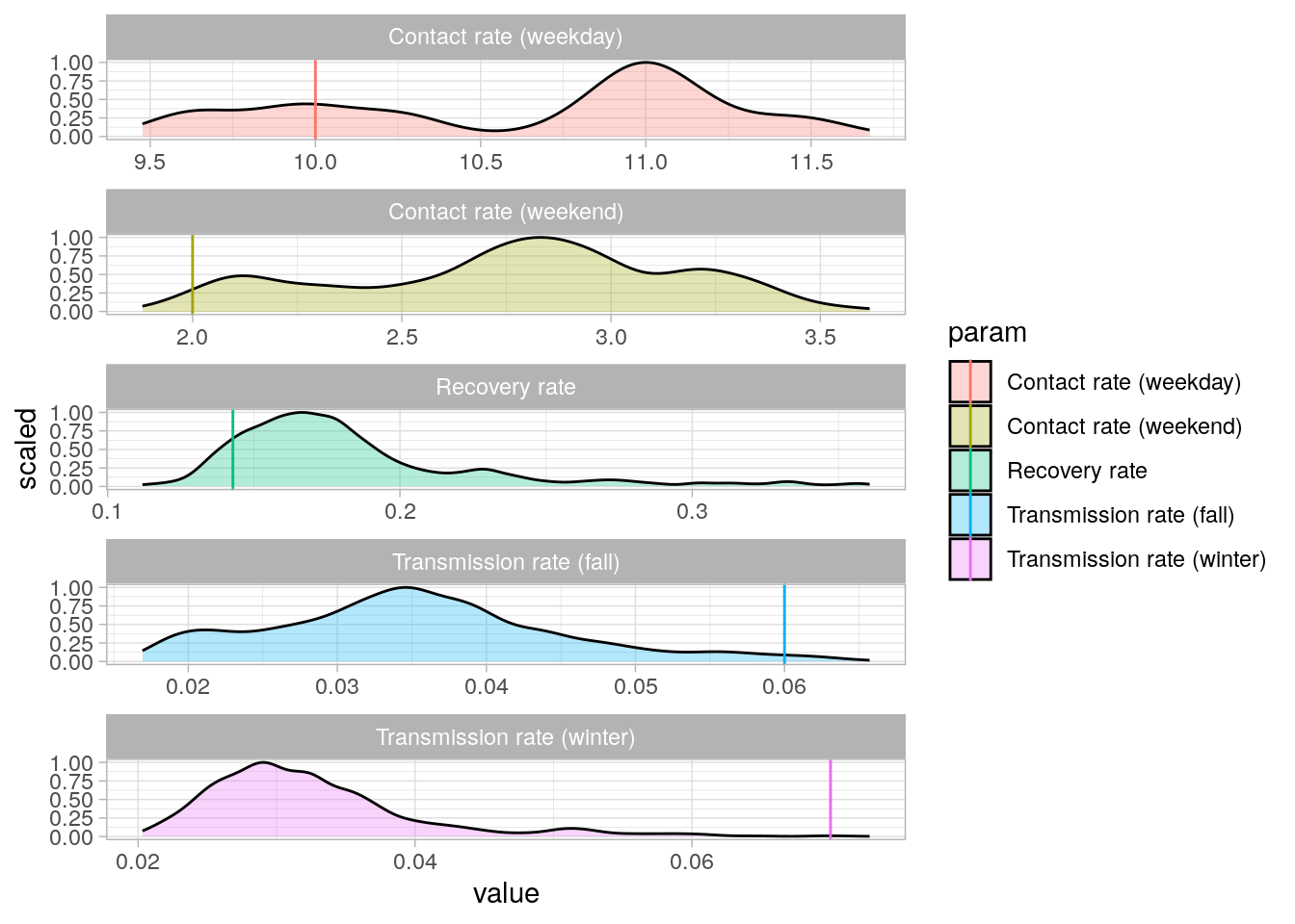
Here is the posterior distribution of the LFMCMC samples with vertical lines representing the initial parameter values.

plot_lfmcmc_post_dist(
  calibration_lfmcmc,
  init_lfmcmc_params,
  param_names,
  seasons
)

We can now run the forecast.

# Create a new SIR CONN model
# - Compute prevalence based on most recent day
forecast_prevalence <- covid_cases[90] / model_n
# - Init the model
covid_sirconn_model <- ModelSIRCONN(
  name              = "COVID-19",
  n                 = model_n,
  prevalence        = forecast_prevalence,
  contact_rate      = init_contact_rate,
  transmission_rate = init_transmission_rate,
  recovery_rate     = init_recovery_rate
)

# Run the simulation for each set of params in the sample
# - Select sample of accepted params from LFMCMC
forecast_sample_n <- 200 # Sample size
params_sample <- get_params_sample(calibration_lfmcmc,
  lfmcmc_n_samples,
  lfmcmc_burnin,
  forecast_sample_n)
# - Set forecast length
model_ndays <- 14
# - Run simulation function for each set of params from the sample
forecast_dist <- apply(params_sample, 1, lfmcmc_simulation_fun)

Our model prevalence is set according to the reported case counts of the most recent day of the UDHHS data. We then take a sample of n = 200 from the LFMCMC accepted parameters (after the burn-in period) and run the SIR connected model with the new prevalence for each set of parameters. Each simulation is for two weeks, giving us a 14-day forecast of COVID-19 in Utah. The forecast mean is shown below along with the 50% and 95% confidence intervals. The actual case counts are plotted in black, while the forecast is plotted in blue.

plot_forecast(forecast_dist, covid_data)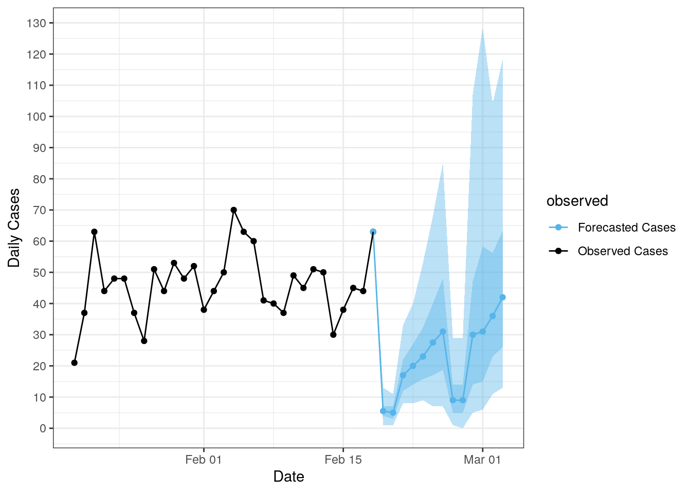

saveRDS(
  list(
    forecast_dist = forecast_dist,
    covid_data = covid_data
  ),
  sprintf(
    "forecast_data_%s.rds",
    format(Sys.time(), "%Y-%m-%d")
  )
)

Technologies

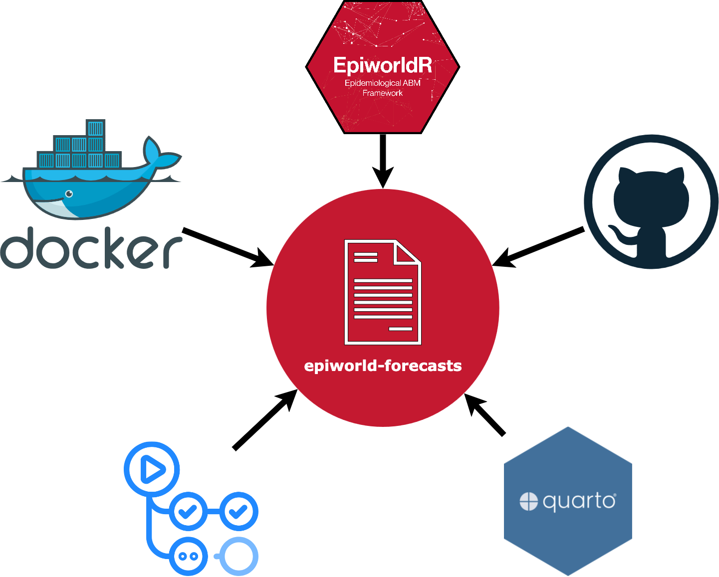
epiworld-forecasts is built with the following technologies:

epiworldR: Fast agent-based modeling R package for disease simulations
Docker: The forecast runs inside a Docker container which has all the needed packages. This container is built in a separate workflow and pushed to the GitHub Container Registry.
GitHub Actions: The forecast runs on a schedule through GitHub Actions
Quarto: Generates the HTML report that is published to GitHub Pages
GitHub: Version control, hosting the source code repository and website