The data.table R package

For most cases, the most proper data wrangling tool in R is the dplyr package. Nonetheless, when dealing with large amounts of data, the data.table package is the fastest alternative available for doing data processing within R (see the benchmarks).

Reading and Writing Data

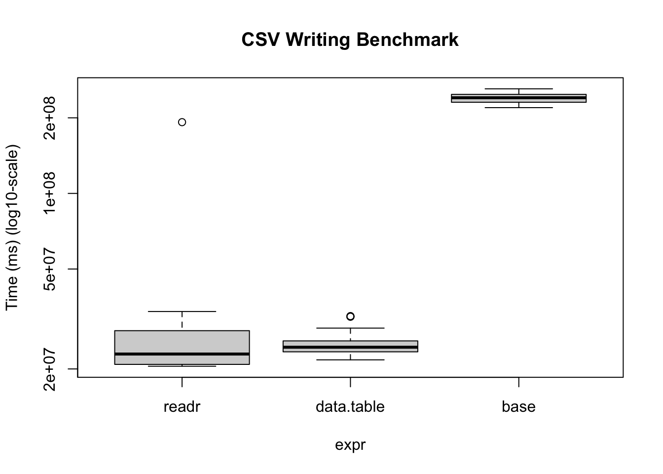
Reading and writing operations with data.table’s fread and fwrite are highly optimized. Here is a benchmark we can do on our own:

library(readr) # tidyverse's
library(data.table)
library(microbenchmark)

# Generating a large dataset of random numbers
set.seed(1231)
x <- runif(5e4 * 10) |> matrix(ncol = 10) |> data.frame()

# Creating tempfiles
temp_dt <- tempfile(fileext = ".csv")
temp_tv <- tempfile(fileext = ".csv")
temp_r  <- tempfile(fileext = ".csv")

bm <- microbenchmark(
  readr      = write_csv(x, temp_tv, num_threads = 1L, progress = FALSE),
  data.table = fwrite(
    x, temp_dt, verbose = FALSE, nThread = 1L,
    showProgress = FALSE),
  base       = write.csv(x, temp_r),
  times = 20
)

Warning in microbenchmark(readr = write_csv(x, temp_tv, num_threads = 1L, :
less accurate nanosecond times to avoid potential integer overflows

bm

Unit: milliseconds
       expr       min        lq      mean    median        uq      max neval
      readr  20.50656  20.85293  32.74184  22.92738  28.40509 192.2000    20
 data.table  21.73935  23.39716  25.49071  24.40361  25.86483  32.4754    20
       base 219.56336 230.62471 239.80889 240.37378 247.95769 260.8928    20

# We can also visualize it
bm |>
  plot(
    log = "y",
    ylab = "Time (ms) (log10-scale)",
    main = "CSV Writing Benchmark"
  )

The same thing applies when reading data

# Writing the data
fwrite(x, temp_r, verbose = FALSE, nThread = 1L, showProgress = FALSE)

# Benchmarking
bm <- microbenchmark(
  readr      = read_csv(
    temp_r, progress = FALSE, num_threads = 1L,
    show_col_types = FALSE
    ),
  data.table = fread(
    temp_r, verbose = FALSE, nThread = 1L,
    showProgress = FALSE
    ),
  base       = read.csv(temp_r),
  times = 10
)

Warning in microbenchmark(readr = read_csv(temp_r, progress = FALSE,
num_threads = 1L, : less accurate nanosecond times to avoid potential integer
overflows

bm

Unit: milliseconds
       expr        min        lq      mean    median        uq       max neval
      readr  40.088898  40.28516  74.29501  41.79661  42.52569 370.04095    10
 data.table   9.947297  10.24852  11.92535  10.63159  11.27336  21.29651    10
       base 148.565591 176.56457 204.73412 199.02650 235.19945 247.29724    10

bm |>
  plot(
    log = "y",
    ylab = "Time (ms) (log10-scale)",
    main = "CSV Reading Benchmark"
  )

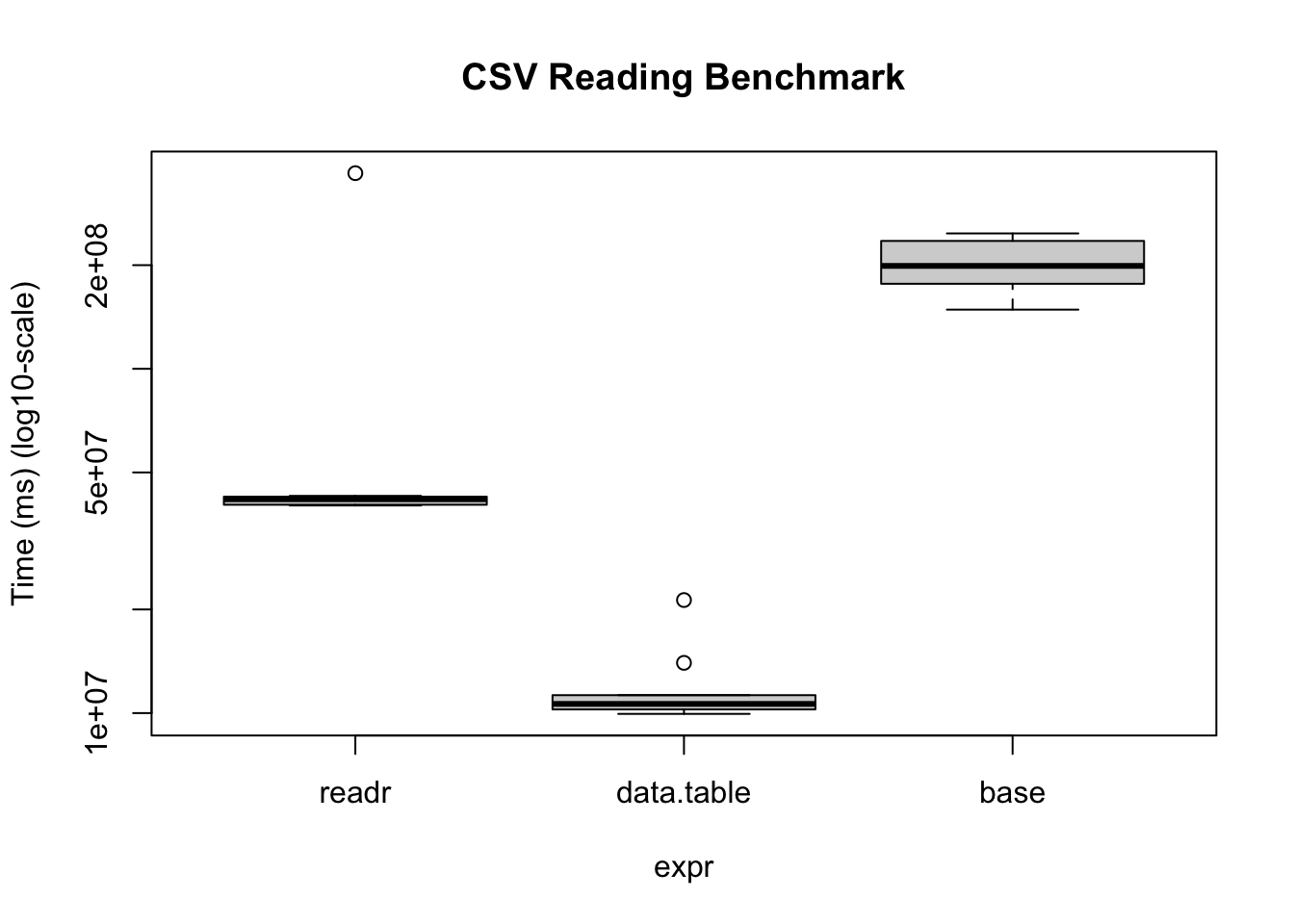
Under the hood, the readr package uses the vroom package. Nonetheless, there are some operations (dealing with character data mostly), where the vroom package shines. Regardless, data.table is a perfect alternative as it goes beyond just reading/writing data.

Example data manipulation

data.table is also the fastest for data manipulation. Here are a couple of examples aggregating data with data table vs dplyr

input <- if (file.exists("flights14.csv")) {
   "flights14.csv"
} else {
  "https://raw.githubusercontent.com/Rdatatable/data.table/master/vignettes/flights14.csv"
}

# Reading the data
flights_dt <- fread(input)
flights_tb <- read_csv(input, show_col_types = FALSE)

library(dplyr)

Attaching package: 'dplyr'

The following objects are masked from 'package:data.table':

    between, first, last

The following objects are masked from 'package:stats':

    filter, lag

The following objects are masked from 'package:base':

    intersect, setdiff, setequal, union

# To avoid some messaging from the function
options(dplyr.summarise.inform = FALSE)

microbenchmark(
  data.table = flights_dt[, .N, by = .(origin, dest)],
  dplyr = flights_tb |>
    group_by(origin, dest) |>
    summarise(n = n())
)

Unit: milliseconds
       expr      min       lq     mean   median       uq       max neval
 data.table 1.788051 2.121955 2.789121 2.367279 2.963931  5.913922   100
      dplyr 5.255011 5.544102 6.682056 5.832742 6.371748 37.637713   100

ForeSITE