Bayesian Transmission Modeling

library(bayestransmission)

Introduction

This package provides a Bayesian framework for transmission modeling on an individual patient level. Modeling is conducted through Markov Chain Monte Carlo (MCMC) methods.This document will explain the basic usage of the package, specification of parameters, and the output of the model.

Data Structure

The algorithms expect a longitudinal data set with the following columns: * facility: The facility where the event occurred. * unit: The unit within the facility where the event occurred. * time: The time at which the event occurred. * patient: The patient involved in the event. * type: The type of event.

The package includes a simulated dataset, simulated.data.

pillar::glimpse(simulated.data)
#> Rows: 8,360
#> Columns: 5
#> $ facility <int> 1, 1, 1, 1, 1, 1, 1, 1, 1, 1, 1, 1, 1, 1, 1, 1, 1, 1, 1, 1, 1…
#> $ unit     <int> 1, 1, 1, 1, 1, 1, 1, 1, 1, 1, 1, 1, 1, 1, 1, 1, 1, 1, 1, 1, 1…
#> $ time     <dbl> 0.060978, 0.061978, 1.560978, 2.883323, 2.884323, 1.422631, 1…
#> $ patient  <int> 1, 1, 1, 1, 1, 10, 10, 10, 10, 19, 19, 19, 23, 23, 23, 28, 28…
#> $ type     <int> 0, 1, 10, 1, 3, 0, 1, 1, 3, 0, 1, 3, 0, 1, 3, 0, 1, 1, 3, 0, …

There are 12 different types of events that can be specified in the type column. These are, expected numerical codes shown in parentheses:

Admission (0) and Discharge (3)
Surveillance Testing Results
- Negative Test (1)
- Positive Test (2)
Clinical Testing Results
- Negative Test (4)
- Positive Test (5)
Generic Testing
- Negative Test (7)
- Positive Test (8)
Antibiotic Use
- single dose (9)
- Start (10)
- Stop (11)
Isolation Procedures
- Start (6)
- Stop (7)

Not all events need to be used in every data set, but the model selected should reflect the data that is available. Care should be taken to correctly code the data. The EventToCode and CodeToEvent functions can be used to convert between.

table(CodeToEvent(simulated.data$type))
#> 
#>      abxoff       abxon   admission   discharge negsurvtest possurvtest 
#>         297         725        2183        2183        2749         223

Model Specifiction

Model Choice

Since the model is implemented in C++ for speed and efficiency, only the specified models can be used. The currently implemented models are:

"LinearAbxModel", A Linear model with antibiotic use as a covariate.
"MixedModel", and
"LogNormalModel"

Model specification and all parameters are controlled through constructor functions of the same name, or generically through the LogNormalModelParams() function.

For all models there is the choice of either a 2 state (susceptible and colonized) or 3 state (susceptible, colonized, and recovered or latent) model. Number of states is set through the nstates parameter, and the number of states in the model overrides what may be specified in any individual component.

Parameters

The remainder of the parameters are grouped into the following categories:

Abx, Antibiotic use,
AbxRate, Antibiotic rates,
InUnit, In unit infection rates,
OutOfUnitInfection, Out of unit infection rates,
Insitu, In situ parameters,
Testing:
- SurveilenceTest, Surveillance testing,
- ClinicalTest, Clinical testing.

Unless otherwise specified the parameters are all distributed gamma with specified shape and rate parameters. Each parameter can also be left as fixed or be sampled at each iteration of the MCMC.

Specifying parameters

Parameters for the model may be specified by the Param() function. This function takes up to four arguments:

1. `init`, is the initial value of the parameter.
2. `weight`, is the weight of the prior distribution in updates.
3. `update`, a flag of if the parameter should be sampled in the MCMC algorithm. 
    `FALSE` indicates that the parameter should be fixed, and is by default `TRUE` when `weight` is greater than zero.
4. `prior`, the mean of the prior distribution.  Taken with the weight will fully parameterize the distribution.

Important: Always explicitly specify init values for parameters to ensure reproducibility and avoid potential numerical issues.

# Fully specified parameter.
Param(init = 0, weight = 1, update = TRUE, prior = 0.5)
# Fixed parameter with explicit init
# Weight = 0 implies update=FALSE and prior is ignored.
Param(init = 0, weight = 0)
# Updated parameter that starts at zero.
Param(init = 0, weight = 1, update = TRUE)
# Short form for fixed parameter
Param(init = 0, weight = 0)

`Abx` Antibiotic use

Antibiotic use is specified by the Abx parameter. This parameter is a list constructed with the AbxParams() function with the following components:

onoff, If antibiotics are being used or not. The two following parameters are only used if onoff is TRUE.
delay, the delay for the antibiotic to take effect.
life, the duration where the antibiotic to be effective.

abx <- AbxParams(onoff = 0, delay = 0.0, life = 2.0)

Currently, all antibiotics are assumed to be equally effective and have the same duration of effectiveness. Note: onoff = 0 means antibiotics are turned off for this example (set to 1 to enable).

`AbxRate` Antibiotic rates

The AbxRate parameter control the antibiotic administration rates.

abxrate <- AbxRateParams(
  # Fixed parameters when antibiotics are off
  uncolonized = Param(init = 1.0, weight = 0),
  colonized = Param(init = 1.0, weight = 0)
)

Here since both parameters are non-zero both will be updated. A rate of zero for either would indicate that group would never be on antibiotics. When antibiotics are turned off (Abx$onoff = 0), these parameters are typically fixed (weight = 0).

`InUnit` In unit infection rate

Transmission within unit is the main defining characteristic that differentiates models. For example the linear antibiotic model, LinearAbxModel(), is differentiated from the log normal model, LogNormalModelParams() by the use of a ABXInUnitParams() for the InUnit argument rather than the LogNormalInUnitAcquisition() which does not take into account antibiotic use. All in unit transmission is defined in terms of acquisition, progression, and clearance.

Aqcuisition Model

In the base log normal antibiotic model, LogNormalABXInUnitParameters() log acquisition probability is a linear function.

$\log(P(\mathrm{Acq(t)})) = % lognormal_logNormalAbxICP.cpp:68-74 \beta_0 + % logbeta_acq_constant \beta_t (t-t_0) + % logbeta_acq_time \beta_c N_c(t) + % logbeta_acq_col() * ncol + \beta_{ca} N_{ca}(t) + % logbeta_acq_abx_col() * ncolabx + \beta_A A_i(t) + % logbeta_acq_onabx() * onabx + \beta_E E_i(t) % logbeta_acq_everabx() * everabx;$

Where $\beta_\star$ represents the coefficient corresponding to the amounts, $N_c(t)$ represent the total number of colonized patients at time $t$ , $N_{ca}(t)$ the number of colonized on antibiotics, and $A_i(t)$ and $E_i(t)$ represents if patient $i$ is currently or ever on antibiotics.

The linear antibiotic (LinearAbxAcquisitionParams) takes a more complicated form for the acquisition model.

$P(\mathrm{Acq(t)}) = \left[e^{\beta_\mathrm{time}(t-t_0)}\right] \left\{e^{\beta_0} \left[ \left(\frac{\beta_\mathrm{freq}}{P(t)}+(1 - e^{\beta_\mathrm{freq}})\right) e^{\beta_\mathrm{mass}}\left( (N_c(t) - N_{ca}(t)) + e^{\beta_\mathrm{col\_abx}}N_{ca}(t) \right) + 1 - e^{\beta_\mathrm{mass}} \right] \right\} \left[ N_S(t) - N_E(t) + e^{\beta_\mathrm{suss\_ever}}\left(\left(E_i(t)-A_i(t)\right) +A_i(t)e^{\beta_\mathrm{suss\_abx}}\right) \right]$

acquisition <- LinearAbxAcquisitionParams(
    base = Param(init = 0.001, weight = 1),     #< Base acquisition rate (Updated)
    time = Param(init = 1.0, weight = 0),       #< Time effect (Fixed)
    mass = Param(init = 1.0, weight = 1),       #< Mass Mixing (Updated)
    freq = Param(init = 1.0, weight = 1),       #< Frequency/Density effect (Updated)
    col_abx = Param(init = 1.0, weight = 0),    #< Colonized on antibiotics (Fixed)
    suss_abx = Param(init = 1.0, weight = 0),   #< Susceptible on antibiotics (Fixed)
    suss_ever = Param(init = 1.0, weight = 0)   #< Ever on antibiotics (Fixed)  
)

Progression Model

In the 3 state model there is a latent state and the progression model controls how patient transition out of the latent state. The base rate can be affected by currently being on antiboitics or ever being on antbiotcs.

$\log(P(\mathrm{progression})) = \delta_0+\delta_AA_i(t) + \delta_EE_i(t)$ the linear antibiotic model is:

$P(\mathrm{progression}) = e^{\delta_0}\left[1-E_i(t)+e^{\delta_2}\left(E_i(t)-A_i(t)+e^{\delta_1}A_i(t)\right)\right]$

Where here we use $\delta$ for the coefficients, but the notation is the same.

progression <- ProgressionParams(
    rate = Param(init = 0.0, weight = 0),      #< Base progression rate (Fixed for 2-state)
    abx  = Param(init = 1.0, weight = 0),      #< Currently on antibiotics (Fixed)
    ever_abx = Param(init = 1.0, weight = 0)   #< Ever on antibiotics (Fixed)
)

Clearance Model

The clearance model is the same as the progression model in both the log normal and the linear cases, the coefficients however are independent.

clearance <- ClearanceParams(
    rate = Param(init = 0.01, weight = 1),     #< Base clearance rate (Updated)
    abx  = Param(init = 1.0, weight = 0),      #< Currently on antibiotics (Fixed)
    ever_abx = Param(init = 1.0, weight = 0)   #< Ever on antibiotics (Fixed)
)

inunit <- ABXInUnitParams(
  acquisition = acquisition,
  progression = progression,
  clearance   = clearance
)

Out of Unit Importation

The out of unit parameters control the rate at which admissions come in, and which state they enter in.

$\log(P(\mathrm{state}_i \rightarrow \mathrm{state}_j)|t) = P_j - Q_{i,j} e^{-t \sum_i r_i}$

outcol <- OutOfUnitInfectionParams(
  acquisition = Param(init = 0.001, weight = 1),
  clearance = Param(init = 0.01, weight = 0),
  progression = Param(init = 0.0, weight = 0)
)

In Situ

I’m not sure what these parameters do. It’s a set of gamma distributed parameters one for each state. The updates and probabilities are not time dependent.

When updating the rates for each state are sampled from a $gamma(N_i, 1)$ distribution. Then all three are normalized to sum to 1.

insitu <- InsituParams(
  # Starting 90/10 split uncolonized to colonized
  # For 2-state model, latent probability is 0
  probs = c(uncolonized = 0.90,
            latent = 0.0,
            colonized = 0.10),
  # Prior values for Bayesian updating  
  priors = c(1, 1, 1),
  # Which states to update (latent is fixed at 0 for 2-state model)
  doit = c(TRUE, FALSE, TRUE)
)

Testing

There are two types of testing, surveillance, which is conducted routinely at regular intervals such as on admission then every 3 days after, and clinical, where the testing is precipitated by staff, and thus the timing is informative.

Surveillance Testing

The timing of surveillance testing is assumed to not be informative. Therefore, surveillance testing is only parameterized in terms of probability of a positive test given the underlying status. Surveillance test parameters are updated with a sample from a $Beta(N_{s,1}, N_{s,0})$ distribution where $N_{s,1}$ and $N_{s,0}$ are the number of positive and negative tests respectively for state $s$ .

surv <- SurveillanceTestParams(
    # Probability of a positive test when uncolonized (false positive rate)
    # IMPORTANT: Must be > 0 to avoid -Inf likelihood. Use small value like 1e-10.
    # Setting to exactly 0.0 causes log(0) = -Inf if any uncolonized patient tests positive.
    uncolonized = Param(init = 1e-10, weight = 0),
    # Probability of a positive test when colonized (true positive rate/sensitivity)
    # Starting at 0.8, will be updated during MCMC
    colonized = Param(init = 0.8, weight = 1),
    # Latent state (for 2-state model, this is not used but must be specified)
    latent = Param(init = 0.0, weight = 0)
)

Clinical Testing

Since clinical testing time is informative, clinical testing is assumed to be at random within infection stage. The rate of testing within each stage is sampled from a gamma distribution. Sensitivity/Specificity are handled the same as surveillance testing and the likelihood is multiplicative between rate and effectiveness.

clin <- RandomTestParams(
    # Rate of testing when uncolonized
    uncolonized = ParamWRate(
      param = Param(init = 0.5, weight = 0), 
      rate = Param(init = 1.0, weight = 0)
    ),
    # Rate of testing when colonized  
    colonized = ParamWRate(
      param = Param(init = 0.5, weight = 0), 
      rate = Param(init = 1.0, weight = 0)
    ),
    # Latent state (for 2-state model, not used but must be specified)
    latent = ParamWRate(
      param = Param(init = 0.5, weight = 0), 
      rate = Param(init = 1.0, weight = 0)
    )
)

All Together

params <- LinearAbxModel(
  nstates = 2,
  Insitu = insitu,
  SurveillanceTest = surv,
  ClinicalTest = clin,
  OutOfUnitInfection = outcol,
  InUnit = inunit,
  Abx = abx,
  AbxRate = abxrate
)

Running the Model

The model is run through the runMCMC() function. The function takes the following arguments:

data: The data frame with patient event data
modelParameters: The model specification (created above)
nsims: Number of MCMC samples to collect after burn-in
nburn: Number of burn-in iterations (default: 100)
outputparam: Whether to save parameter values at each iteration (default: TRUE)
outputfinal: Whether to save the final model state (default: FALSE)
verbose: Whether to print progress messages (default: FALSE)

system.time(
  results <- runMCMC(
    data = simulated.data_sorted,
    modelParameters = params,
    nsims = 100,
    nburn = 10,
    outputparam = TRUE,
    outputfinal = TRUE,
    verbose = FALSE
  )
)
#>    user  system elapsed 
#>  17.819  16.486  17.159

Analyzing MCMC Results

Converting Parameters to Data Frame

The results$Parameters object contains the MCMC chain of all model parameters. To create trace plots and posterior distributions, we use the mcmc_to_dataframe() function to convert this nested list structure into a tidy data frame format.

# Convert parameters to data frame using package function
param_df <- mcmc_to_dataframe(results)

# Display first few rows
head(param_df)
#>   iteration insitu_uncolonized insitu_colonized surv_test_uncol_neg
#> 1         1          0.4649756       0.53502440               1e-10
#> 2         2          0.8145916       0.18540844               1e-10
#> 3         3          0.1541333       0.84586666               1e-10
#> 4         4          0.9707602       0.02923979               1e-10
#> 5         5          0.8663606       0.13363938               1e-10
#> 6         6          0.4665449       0.53345514               1e-10
#>   surv_test_col_neg surv_test_uncol_pos surv_test_col_pos clin_test_uncol
#> 1         0.8520047               1e-10         0.7868844             0.5
#> 2         0.7822836               1e-10         0.9999999             0.5
#> 3         0.8599913               1e-10         0.6272905             0.5
#> 4         0.8281964               1e-10         0.9998167             0.5
#> 5         0.7709993               1e-10         0.4185874             0.5
#> 6         0.8377648               1e-10         0.9998530             0.5
#>   clin_test_col clin_rate_uncol clin_rate_col outunit_acquisition
#> 1           0.5               1             1         0.001181636
#> 2           0.5               1             1         0.001181636
#> 3           0.5               1             1         0.001181636
#> 4           0.5               1             1         0.001181636
#> 5           0.5               1             1         0.001181636
#> 6           0.5               1             1         0.001181636
#>   outunit_clearance  inunit_base inunit_time inunit_mass inunit_freq
#> 1              0.01 0.0008107566           1           1           1
#> 2              0.01 0.0006954064           1           1           1
#> 3              0.01 0.0006984290           1           1           1
#> 4              0.01 0.0007232861           1           1           1
#> 5              0.01 0.0008540253           1           1           1
#> 6              0.01 0.0008682528           1           1           1
#>   inunit_colabx inunit_susabx inunit_susever  inunit_clr inunit_clrAbx
#> 1             1             1              1 0.008567051             1
#> 2             1             1              1 0.007480784             1
#> 3             1             1              1 0.006921057             1
#> 4             1             1              1 0.006731989             1
#> 5             1             1              1 0.005782676             1
#> 6             1             1              1 0.005212212             1
#>   inunit_clrEver abxrate_uncolonized abxrate_colonized loglikelihood
#> 1              1                   1                 1     -13020.82
#> 2              1                   1                 1     -13024.24
#> 3              1                   1                 1     -13033.93
#> 4              1                   1                 1     -13007.50
#> 5              1                   1                 1     -13025.07
#> 6              1                   1                 1     -13054.66

Trace Plots

Trace plots show the evolution of parameters across MCMC iterations, helping to assess convergence.

library(ggplot2)
library(tidyr)

# Select key parameters for trace plots
trace_params <- param_df[, c("iteration", "insitu_colonized", "surv_test_col_pos", 
                              "outunit_acquisition", "inunit_base", 
                              "abxrate_colonized", "loglikelihood")]

# Convert to long format
trace_long <- pivot_longer(trace_params, 
                           cols = -iteration,
                           names_to = "parameter",
                           values_to = "value")

# Create trace plots
ggplot(trace_long, aes(x = iteration, y = value)) +
  geom_line() +
  facet_wrap(~parameter, scales = "free_y", ncol = 2) +
  theme_minimal() +
  labs(title = "MCMC Trace Plots",
       x = "Iteration",
       y = "Parameter Value")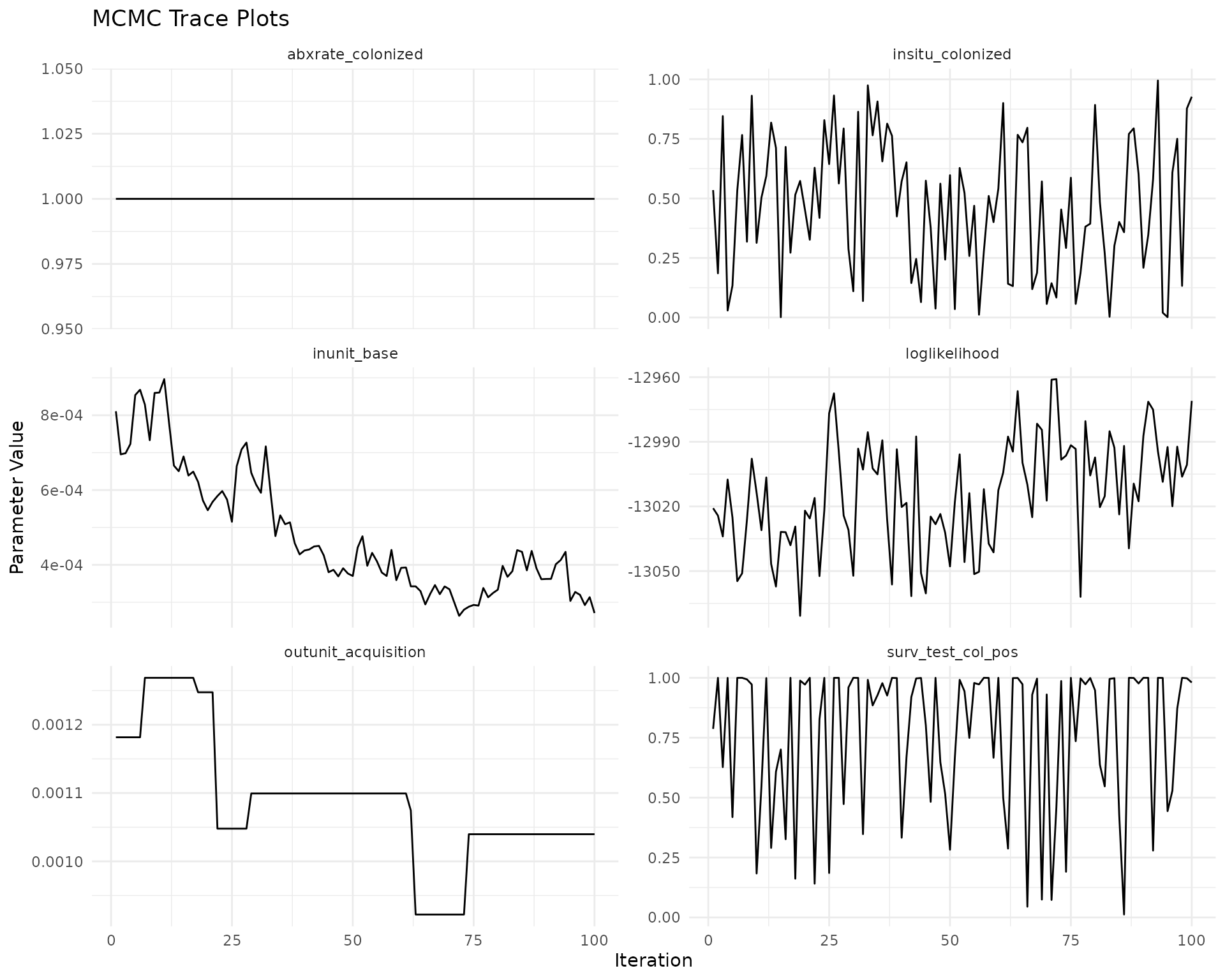

Posterior Distributions

Posterior distributions show the estimated distribution of each parameter after the MCMC sampling.

# Remove burn-in if needed (here we already set nburn in the MCMC call)
# For demonstration, let's use all samples since nburn=0 was specified

# Create density plots for posterior distributions
ggplot(trace_long, aes(x = value)) +
  geom_density(fill = "steelblue", alpha = 0.5) +
  geom_vline(aes(xintercept = mean(value, na.rm = TRUE)), 
             color = "red", linetype = "dashed") +
  facet_wrap(~parameter, scales = "free", ncol = 2) +
  theme_minimal() +
  labs(title = "Posterior Distributions",
       subtitle = "Red dashed line shows posterior mean",
       x = "Parameter Value",
       y = "Density")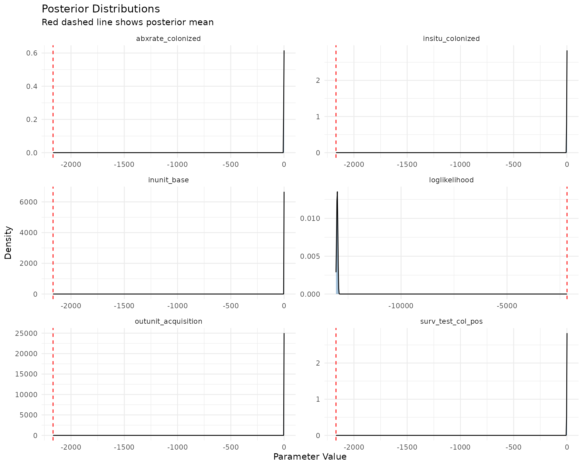

Summary Statistics

# Calculate summary statistics for each parameter
library(dplyr)
#> 
#> Attaching package: 'dplyr'
#> The following objects are masked from 'package:stats':
#> 
#>     filter, lag
#> The following objects are masked from 'package:base':
#> 
#>     intersect, setdiff, setequal, union

summary_stats <- trace_long %>%
  group_by(parameter) %>%
  summarise(
    mean = mean(value, na.rm = TRUE),
    median = median(value, na.rm = TRUE),
    sd = sd(value, na.rm = TRUE),
    q025 = quantile(value, 0.025, na.rm = TRUE),
    q975 = quantile(value, 0.975, na.rm = TRUE),
    .groups = "drop"
  )

print(summary_stats)
#> # A tibble: 6 × 6
#>   parameter                    mean        median         sd      q025      q975
#>   <chr>                       <dbl>         <dbl>      <dbl>     <dbl>     <dbl>
#> 1 abxrate_colonized        1             1         0           1   e+0  1    e+0
#> 2 insitu_colonized         0.466         0.494     0.285       7.16e-3  9.32 e-1
#> 3 inunit_base              0.000480      0.000430  0.000167    2.84e-4  8.60 e-4
#> 4 loglikelihood       -13014.       -13015.       25.5        -1.31e+4 -1.30 e+4
#> 5 outunit_acquisition      0.00109       0.00110   0.0000951   9.22e-4  1.27 e-3
#> 6 surv_test_col_pos        0.766         0.966     0.304       7.37e-2  1.000e+0